
Beginner
LunaBench introduces a comprehensive benchmarking framework designed to assess your algorithms or use cases against the state-of-the-art solutions available in quantum, hybrid, and classical environments. With LunaBench, you can determine the competitiveness of your algorithm and explore the potential quantum advantage for your specific use case.
Problem Description
The Binary Paint Shop Problem in Automotive Manufacturing
The Binary Paint Shop Problem, significant in the automotive industry, is a theoretical yet practical challenge in manufacturing optimization. In car factories, vehicles are painted in one of two colors post-assembly. The core issue arises when consecutive cars require different colors, necessitating a time and resource-intensive process for the painting robots to switch colors. This includes rinsing, nozzle cleaning, and reapplying a new color, leading to increased costs and inefficiency.
The sequence of car assembly is fixed, but there's flexibility in choosing the paint color for the first car in each pair, dictating the color for the second car. This decision impacts resource use and process efficiency. Similar to the Traveling Salesperson Problem (TSP) in logistics, solving the Binary Paint Shop Problem could lead to significant improvements in manufacturing processes, akin to how TSP optimized route planning.
# define the problem type
problem_name = "bpsp"

Given a sequence of cars, you can represent it as a list where each number corresponds to a specific type of car:
For benchmarking purposes, LunaBench will utilize three different instances. These instances will be input as a dataset in a dictionary format, where each key represents a unique instance identifier and its corresponding value denotes the specific problem configuration.
In this scenario, LunaBench will be responsible for managing all aspects of the mathematical modeling.
# define the dataset
dataset = {
    "id_00": {"sequence": [1, 2, 0, 1, 2, 0]},
    "id_01": {"sequence": [1, 0, 0, 1, 2, 2]},
    "id_02": {"sequence": [0, 1, 0, 1, 2, 2]},
}
Choosing Algorithms
LunaBench provides an extensive collection of pre-configured algorithms designed for tackling optimization challenges. This tutorial will focus on demonstrating the fundamental applications of LunaBench through the use of Simulated Annealing (sa) and Quantum Approximate Optimization Algorithm (qaoa). For additional information on a broader spectrum of algorithms, encompassing quantum, hybrid, classical, and custom options, please consult our comprehensive list available on LunaBench GitHub. To get access, please contact us here.
For a statistically significant evaluation of the algorithms' performance, you can define the number of runs for each algorithm. This method ensures a thorough and accurate measurement of their effectiveness in different scenarios.
# specify the algorithms and number of runs for each algorithm
algorithms = ["sa", "qaoa"]
n_runs = 3
Solving the dataset
The successful configuration of the BPSP dataset and algorithms has paved the way to address the entire dataset comprehensively. This can be achieved by importing the solve_dataset function from the LunaBench package, which enables the solving of the dataset. Upon completion, the results, accompanied by supplementary information, will be conveniently available in the designated CSV file located at luna_results/{$dataset_name}/solve/{$result_id}/solutions.csv . Please note that, by default, both dataset_name and result_id are configured to have matching time identifiers.
from lunabench import solve_dataset

# solve the complete dataset
solved, result_id = solve_dataset(
    problem_name=problem_name,
    dataset=dataset,
    solve_algorithms=algorithms,
    n_runs=n_runs,
)
Evaluating the solutions
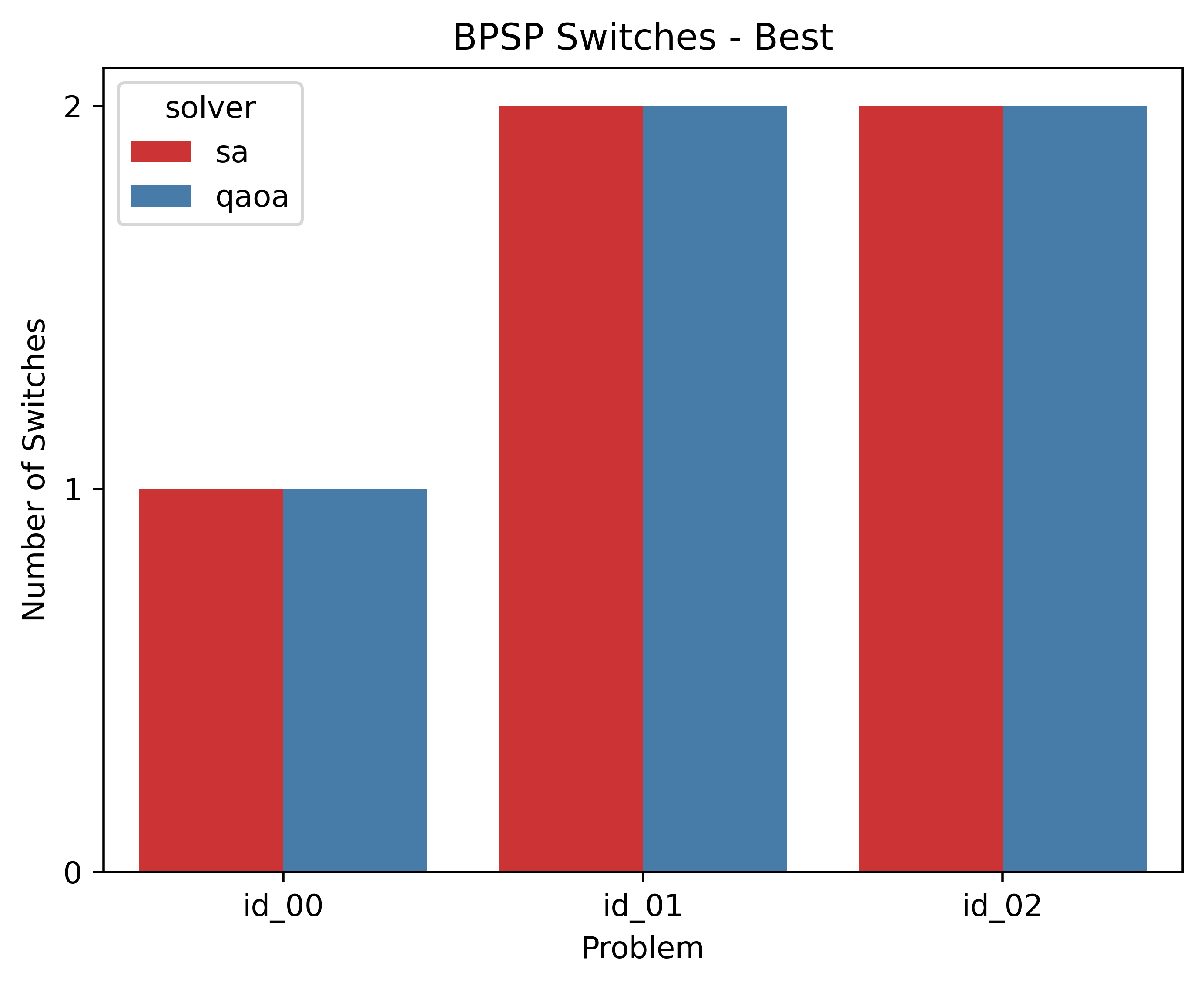
LunaBench provides predefined metrics to assess and compare the performance of various algorithms. Specifically, for the BPSP, the metric of interest is the number of switches in the best solution produced by each algorithm. This comparison is facilitated by employing bpsp_n_switches as the chosen metric. Utilizing the evaluate_results function, you can easily obtain the computed metric for each problem instance, enabling a straightforward comparison of algorithmic performance. The results of this evaluation are conveniently compiled in a CSV file, which can be accessed at luna_results/{$dataset_name}/eval/{$result_id}/results.csv.
from lunabench import evaluate_results

# define the metrics
metrics = ["bpsp_n_switches"]

# run the evaluation
eval_data, plot_outs = evaluate_results(result_id=result_id, dataset=dataset, metrics_config=metrics)
Plotting the results
LunaBench provides an intuitive way to compare evaluation results through user-friendly plots. These visual comparisons can be accessed in the luna_results/{$dataset_name}/eval/{$result_id}/ directory.
import os
from IPython.display import SVG

# display the metric plot
display(
    SVG(
        filename=os.path.join(
            os.getcwd(),
            "luna_results",
            result_id,
            "eval",
            result_id,
            "best_switches.svg",
        )
    )
)
Customizing the execution
In the upcoming "Intermediate" chapter, the focus shifts towards optimizing custom problems, spanning from QUBOs to Qiskit Circuits. This section delves into tailoring execution parameters to meet specific requirements.
For those keen on implementing custom algorithms and assessing outcomes through customized metrics, the "Expert" tutorial chapter offers comprehensive guidance. This segment is designed to equip you with the knowledge to execute your algorithms effectively and evaluate results with precision using LunaBench.