Benchmarking Optimization Problems via the Use Case and Algorithm Libraries
In this tutorial, you'll engage with LunaBench to solve the Binary Paint Shop Problem (BPSP), navigating through dataset creation, algorithm selection, benchmark execution, result evaluation, and result visualization. This guide is perfect for those stepping into benchmarking optimization problems.
Before we begin, ensure you have installed the LunaBench Python SDK.
Upon completing this tutorial, you will be able to:
- Create a dataset of problem instances using our use case library.
- Set up the algorithms to be used for benchmarking using our algorithm library.
- Running a benchmark pipeline using LunaBench.
- Evaluate the benchmark results using pre-defined use case metrics.
- Plotting the benchmark results via use case metrics.
Example: The Binary Paint Shop Problem in Automotive Manufacturing
The Binary Paint Shop Problem is an intriguing challenge that holds particular relevance in the automotive manufacturing sector. It's a practical issue faced during the optimization of manufacturing lines. In car production facilities, each vehicle is painted with one of two colors after assembly.
The problem mainly occurs when there's a need to switch colors for consecutive cars, leading to a substantial increase in time and resources due to the required cleaning and preparation for the new color. This includes tasks like rinsing, cleaning the nozzles, and applying the new paint, all of which contribute to higher costs and lower efficiency.
While the assembly sequence of the cars is predetermined, there's an opportunity to choose the paint color for the first car in each pair. This choice influences the overall resource consumption and the efficiency of the painting process.
Much like the Traveling Salesperson Problem (TSP) revolutionized logistics with optimized route planning, effectively tackling the Binary Paint Shop Problem could lead to marked enhancements in manufacturing efficiency.

Imagine you have a series of cars coming off the assembly line, and you need to decide their paint colors. This sequence can be represented as a simple list, where each number stands for a different car model:
For the sake of this tutorial, we're going to experiment with three distinct scenarios. We'll present these scenarios as a dataset within a dictionary, where every key is a unique identifier for each scenario, and the value is the lineup of cars for that particular problem.
This approach gives us a clear view of the problem at hand. However, to make this information usable for algorithms, especially in the realm of quantum optimization, we need to translate it into a mathematical structure. This is where the Quadratic Unconstrained Binary Optimization (QUBO) model comes into play. Fortunately, if you're utilizing problems from our use case library, you don't have to worry about this translation. LunaBench automatically takes care of converting your problem into the necessary QUBO format, making your life much easier.
# Define the problem type
problem_name = "bpsp"

# Define the dataset
dataset = {
    "id_00": {"sequence": [1, 2, 0, 1, 2, 0]},
    "id_01": {"sequence": [1, 0, 0, 1, 2, 2]},
    "id_02": {"sequence": [0, 1, 0, 1, 2, 2]},
}
2. Selecting Algorithms for Benchmarking
LunaBench provides a wide array of algorithms ready to tackle various optimization tasks. In this tutorial, we're highlighting the basics of LunaBench through two specific approaches: Simulated Annealing (SA) and the Quantum Approximate Optimization Algorithm (QAOA). These algorithms represent classical and quantum strategies, respectively, offering a glimpse into the diverse toolkit LunaBench provides.
For those interested in exploring a wider range of algorithms — including quantum, hybrid, classical, and even custom-made solutions — our extensive collection is detailed on the LunaBench GitHub page. Access is available upon request here.
For a statistically significant evaluation of the algorithms' performance, you can define the number of runs for each algorithm. This method ensures a thorough and accurate measurement of their effectiveness in different scenarios.
# Specify the algorithms and number of runs for each algorithm
algorithms = ["sa", "qaoa"]
n_runs = 3
3. Launching the Benchmark Pipeline
With the Binary Paint Shop Problem dataset and our selected algorithms ready, we're now set to tackle the problem across all instances. This step involves utilizing LunaBench's capabilities to systematically work through the dataset. Instead of directly calling specific functions, think of this as instructing LunaBench to apply our chosen algorithms - SA and QAOA — to each scenario within our dataset.
from lunabench import solve_dataset

# Solve the entire dataset using your chosen algorithms
solved, result_id = solve_dataset(
    problem_name=problem_name,
    dataset=dataset,
    solve_algorithms=algorithms,
    n_runs=n_runs
)
Upon finishing the benchmarking process, you'll find the outcomes, along with additional details, neatly organized in a CSV file. This file is accessible at luna_results/{$dataset_name}/solve/{$result_id}/solutions.csv. It's designed so that both the dataset name and the result ID align with the same time identifiers by default.
This setup ensures easy tracking and organization of your results, making it straightforward to review and analyze the performance of the algorithms across different instances of the problem.
from lunabench import evaluate_results

# Define the metric to be used
metrics = ["bpsp_n_switches"]

# Run the evaluation
eval_data, plot_outs = evaluate_results(result_id=result_id, dataset=dataset, metrics_config=metrics)

print(eval_data)
Output:
      id solver                      bpsp_n_switches
0  id_00     sa  [1, [0.0, 0.0, 0.0, 1.0, 1.0, 1.0]]
1  id_00   qaoa  [1, [1.0, 1.0, 1.0, 0.0, 0.0, 0.0]]
2  id_01     sa  [2, [1.0, 1.0, 0.0, 0.0, 0.0, 1.0]]
3  id_01   qaoa  [2, [0.0, 0.0, 1.0, 1.0, 1.0, 0.0]]
4  id_02     sa  [2, [0.0, 0.0, 1.0, 1.0, 1.0, 0.0]]
5  id_02   qaoa  [2, [0.0, 0.0, 1.0, 1.0, 1.0, 0.0]]
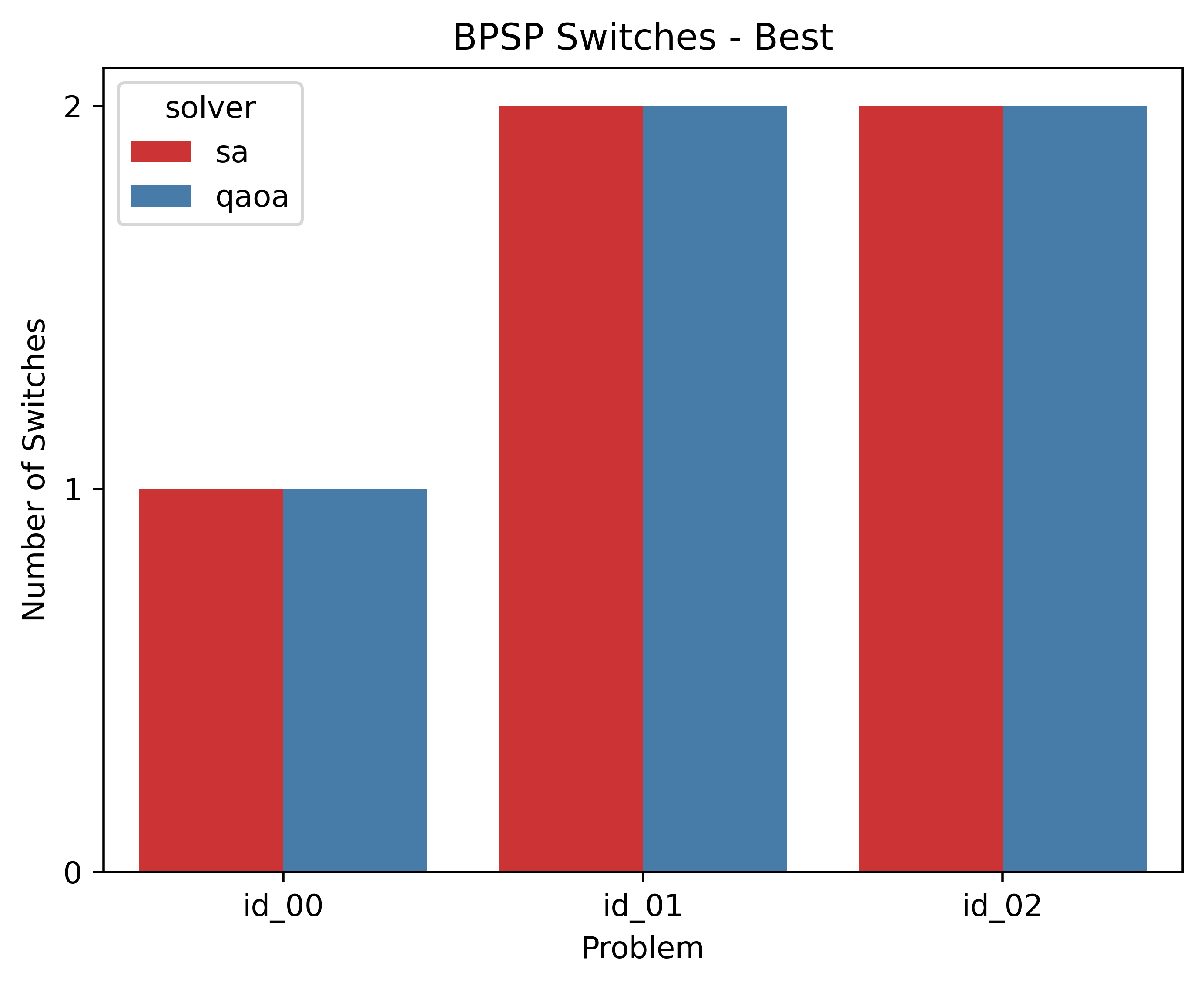
5. Plotting the Benchmark Results
LunaBench offers a straightforward and engaging method to visualize and compare the outcomes of your benchmarks. By generating user-friendly plots, it simplifies the analysis, allowing for an intuitive understanding of how different algorithms perform against each other. You can find these visual comparisons in the luna_results/{$dataset_name}/eval/{$result_id} directory, where each plot gives you a clear visual representation of the algorithms' efficiency and performance across the scenarios tested.
import os
from IPython.display import SVG

# Display the metric plot
display(
    SVG(
        filename=os.path.join(
            os.getcwd(),
            "luna_results",
            result_id,
            "eval",
            result_id,
            "best_switches.svg"
        )
    )
)
Output: