Minimal Spanning Tree Example

Download Notebook

The Minimum Spanning Tree problem finds the minimum-weight subset of edges connecting all nodes without forming cycles. Classical algorithms (Kruskal, Prim) solve it in polynomial time; the QUBO formulation enables quantum approaches.

import getpass
import os

import numpy as np
from dotenv import load_dotenv
from luna_quantum.algorithms import SCIP

from luna_usecases.minimal_spanning_tree import (
    MinimalSpanningTreeCollection,
    MinimalSpanningTreeData,
    MinimalSpanningTreeFormulation,
    MinimalSpanningTreeInstance,
)

load_dotenv()
if "LUNA_API_KEY" not in os.environ:
    os.environ["LUNA_API_KEY"] = getpass.getpass("Enter your Luna API key: ")

Create Data

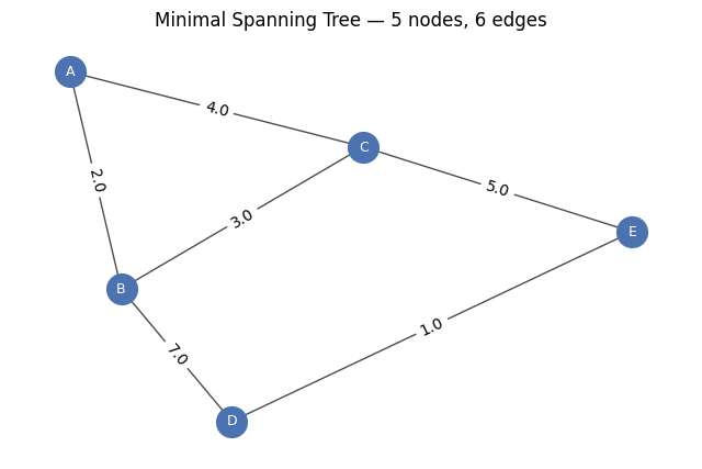
Define a 5-node weighted graph. Edge weights represent connection costs.

adj = np.array(
    [
        [0, 2, 4, 0, 0],
        [2, 0, 3, 7, 0],
        [4, 3, 0, 0, 5],
        [0, 7, 0, 0, 1],
        [0, 0, 5, 1, 0],
    ]
)
node_names = ["A", "B", "C", "D", "E"]
data = MinimalSpanningTreeData.from_adjacency_matrix(adjacency_matrix=adj, node_names=node_names)
print(data.to_string())

Minimal Spanning Tree Data:
  Nodes: 5
  Edges: 6

Plot Data

Visualize the weighted graph.

data.plot()

<Axes: title={'center': 'Minimal Spanning Tree — 5 nodes, 6 edges'}>

Create Formulation

Select edges that connect all nodes with minimum total weight and no cycles.

formulation = MinimalSpanningTreeFormulation()
print(formulation.to_string(data))

Minimal Spanning Tree Formulation:
  Nodes: 5
  Edges: 6

Decision Variables:
  y[i,j] in {0,1} for each edge (i,j)
  y[i,j] = 1 if edge (i,j) is in the tree
  f[i,j], f[j,i] in {0, ..., 4} for each edge (i,j)
  f[i,j] = directed flow on edge from i to j
  Total: 6 binary + 12 integer = 18 variables

Objective:
  minimize sum_False w_ij * y[i,j]

Constraints:
  1. Exactly n-1 edges selected (1 constraint):
     sum_{(i,j)} y[i,j] == 4
  2. Flow conservation at non-root nodes (4 constraints):
     sum_j f[j,v] - sum_j f[v,j] == 1  for all v != root
  3. Flow capacity (6 constraints):
     f[i,j] + f[j,i] <= 4 * y[i,j]  for all edges (i,j)
  4. Root sends n-1 units of flow (1 constraint):
     sum_j f[root,j] - sum_j f[j,root] == 4
  5. Flow bounds (24 constraints):
     0 <= f[i,j] <= 4  for all directed edges

Create Instance

Combine data and formulation into a solvable instance.

instance = MinimalSpanningTreeInstance(data=data, formulation=formulation)
print(instance.to_string())

Data:Minimal Spanning Tree Data:
  Nodes: 5
  Edges: 6
Formulation:Minimal Spanning Tree Formulation:
  Nodes: 5
  Edges: 6

Decision Variables:
  y[i,j] in {0,1} for each edge (i,j)
  y[i,j] = 1 if edge (i,j) is in the tree
  f[i,j], f[j,i] in {0, ..., 4} for each edge (i,j)
  f[i,j] = directed flow on edge from i to j
  Total: 6 binary + 12 integer = 18 variables

Objective:
  minimize sum_False w_ij * y[i,j]

Constraints:
  1. Exactly n-1 edges selected (1 constraint):
     sum_{(i,j)} y[i,j] == 4
  2. Flow conservation at non-root nodes (4 constraints):
     sum_j f[j,v] - sum_j f[v,j] == 1  for all v != root
  3. Flow capacity (6 constraints):
     f[i,j] + f[j,i] <= 4 * y[i,j]  for all edges (i,j)
  4. Root sends n-1 units of flow (1 constraint):
     sum_j f[root,j] - sum_j f[j,root] == 4
  5. Flow bounds (24 constraints):
     0 <= f[i,j] <= 4  for all directed edges

Formulate Model

Translate the instance into a mathematical optimization model.

model = instance.formulate()

Solve and Interpret

Solve the model with SCIP and interpret the raw result into a use-case-specific solution.

scip = SCIP()
job = scip.run(model)
sol = job.result()
uc_solution = instance.interpret(sol)
print(uc_solution.to_string())

/Users/maximilianjanetschek/PycharmProjects/luna-usecases/.venv/lib/python3.13/site-packages/rich/live.py:260:
UserWarning: install "ipywidgets" for Jupyter support
  warnings.warn('install "ipywidgets" for Jupyter support')

2026-05-29 11:35:18 INFO     Sleeping for 5.0 seconds. Waiting and checking a function in a loop.

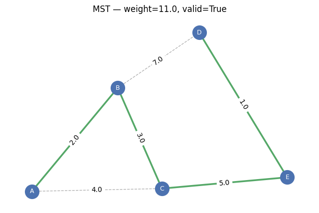
Minimal Spanning Tree Solution:
  Total weight: 11.0
  Valid: True
  Tree edges: [('A', 'B'), ('B', 'C'), ('C', 'E'), ('D', 'E')]

Plot Solution

Visualize the optimal solution.

uc_solution.plot(data)

<Axes: title={'center': 'MST — weight=11.0, valid=True'}>

Collections

Generate a benchmark collection of random instances for batch processing.

collection = MinimalSpanningTreeCollection.from_random(
    min_nodes=4,
    max_nodes=6,
    num_instances=2,
    seed=42,
)
model = collection.instances[0].formulate()
print(model)

Model: minimal_spanning_tree<minimal_spanning_tree>
Minimize
  7.903351786733379 * y_0_1 + 1.6214616397519919 * y_0_2
  + 9.3202717031276 * y_0_3 + 2.248919008072832 * y_1_3
Subject To
  n_minus_1_edges: y_0_1 + y_0_2 + y_0_3 + y_1_3 == 3
  flow_conservation_1: f_0_1 - f_1_0 - f_1_3 + f_3_1 == 1
  flow_conservation_2: f_0_2 - f_2_0 == 1
  flow_conservation_3: f_0_3 - f_3_0 + f_1_3 - f_3_1 == 1
  flow_capacity_0_1: -3 * y_0_1 + f_0_1 + f_1_0 <= 0
  flow_capacity_0_2: -3 * y_0_2 + f_0_2 + f_2_0 <= 0
  flow_capacity_0_3: -3 * y_0_3 + f_0_3 + f_3_0 <= 0
  flow_capacity_1_3: -3 * y_1_3 + f_1_3 + f_3_1 <= 0
  root_flow: f_0_1 - f_1_0 + f_0_2 - f_2_0 + f_0_3 - f_3_0 == 3
Bounds
  0 <= f_0_1 <= 3
  0 <= f_1_0 <= 3
  0 <= f_0_2 <= 3
  0 <= f_2_0 <= 3
  0 <= f_0_3 <= 3
  0 <= f_3_0 <= 3
  0 <= f_1_3 <= 3
  0 <= f_3_1 <= 3
Binary
  y_0_1 y_0_2 y_0_3 y_1_3
Integer
  f_0_1 f_1_0 f_0_2 f_2_0 f_0_3 f_3_0 f_1_3 f_3_1