Uncapacitated Facility Location Problem (UFLP) Example
The Uncapacitated Facility Location Problem (UFLP) asks which facilities to open and how to assign customers to minimize the total cost of opening facilities plus transporting goods. Each facility has a fixed opening cost and unlimited capacity.
import getpass
import os

import matplotlib.pyplot as plt
from dotenv import load_dotenv
from luna_quantum.algorithms import SCIP

from luna_usecases.uncapacitated_facility_location_problem import (
    UflpCollection,
    UflpData,
    UflpFormulation,
    UflpInstance,
)

load_dotenv()
if "LUNA_API_KEY" not in os.environ:
    os.environ["LUNA_API_KEY"] = getpass.getpass("Enter your Luna API key: ")
Create Data
Define a small instance with 3 potential warehouse locations and 5 customers. Each facility has a fixed opening cost and there is a per-unit transport cost from each customer to each facility.
data = UflpData.from_cost_matrix(
    facility_costs=[100.0, 150.0, 120.0],
    transport_costs=[
        [10.0, 30.0, 25.0],  # customer 0
        [25.0, 10.0, 30.0],  # customer 1
        [15.0, 25.0, 10.0],  # customer 2
        [20.0, 15.0, 25.0],  # customer 3
        [30.0, 20.0, 15.0],  # customer 4
    ],
)
print(data.to_string())
Uncapacitated Facility Location Problem:
  Facilities: 3
  Customers: 5
  Facility costs: ['100.0', '150.0', '120.0']
  Transport cost range: [10.0, 30.0]
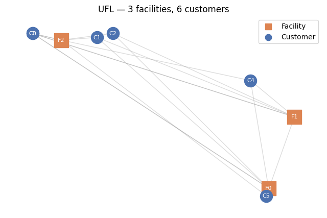
Plot Data
Visualize the problem as a bipartite graph with facilities on the left and customers on the right. If positions are povided, actual positions are plotted
Create Formulation
Set up binary decision variables for facility opening and customer assignment.
Uncapacitated Facility Location Formulation:
  Facilities: 3
  Customers: 5

Decision Variables:
  y_j ∈ {0,1} for j = 0, ..., 2 (facility opening)
  x_ij ∈ {0,1} for i = 0, ..., 4, j = 0, ..., 2 (assignment)
  Total: 18 binary variables

Objective:
  minimize  Σ_j f_j · y_j  +  Σ_i Σ_j c_ij · x_ij

Constraints:
  1. Assignment: Σ_j x_ij = 1 for all i  (5 constraints)
  2. Linking: x_ij ≤ y_j for all i, j  (15 constraints)
Create Instance
Combine data and formulation into a solvable instance.
Data:Uncapacitated Facility Location Problem:
  Facilities: 3
  Customers: 5
  Facility costs: ['100.0', '150.0', '120.0']
  Transport cost range: [10.0, 30.0]
Formulation:Uncapacitated Facility Location Formulation:
  Facilities: 3
  Customers: 5

Decision Variables:
  y_j ∈ {0,1} for j = 0, ..., 2 (facility opening)
  x_ij ∈ {0,1} for i = 0, ..., 4, j = 0, ..., 2 (assignment)
  Total: 18 binary variables

Objective:
  minimize  Σ_j f_j · y_j  +  Σ_i Σ_j c_ij · x_ij

Constraints:
  1. Assignment: Σ_j x_ij = 1 for all i  (5 constraints)
  2. Linking: x_ij ≤ y_j for all i, j  (15 constraints)
Formulate Model
Translate the instance into a mathematical optimization model.
Model: uncapacitated_facility_location_problem<uncapacitated_facility_location_problem>
Minimize
  100 * y_F0 + 150 * y_F1 + 120 * y_F2 + 10 * x_C0_F0 + 30 * x_C0_F1
  + 25 * x_C0_F2 + 25 * x_C1_F0 + 10 * x_C1_F1 + 30 * x_C1_F2 + 15 * x_C2_F0
  + 25 * x_C2_F1 + 10 * x_C2_F2 + 20 * x_C3_F0 + 15 * x_C3_F1 + 25 * x_C3_F2
  + 30 * x_C4_F0 + 20 * x_C4_F1 + 15 * x_C4_F2
Subject To
  assign_C0: x_C0_F0 + x_C0_F1 + x_C0_F2 == 1
  assign_C1: x_C1_F0 + x_C1_F1 + x_C1_F2 == 1
  assign_C2: x_C2_F0 + x_C2_F1 + x_C2_F2 == 1
  assign_C3: x_C3_F0 + x_C3_F1 + x_C3_F2 == 1
  assign_C4: x_C4_F0 + x_C4_F1 + x_C4_F2 == 1
  link_C0_F0: -y_F0 + x_C0_F0 <= 0
  link_C0_F1: -y_F1 + x_C0_F1 <= 0
  link_C0_F2: -y_F2 + x_C0_F2 <= 0
  link_C1_F0: -y_F0 + x_C1_F0 <= 0
  link_C1_F1: -y_F1 + x_C1_F1 <= 0
  link_C1_F2: -y_F2 + x_C1_F2 <= 0
  link_C2_F0: -y_F0 + x_C2_F0 <= 0
  link_C2_F1: -y_F1 + x_C2_F1 <= 0
  link_C2_F2: -y_F2 + x_C2_F2 <= 0
  link_C3_F0: -y_F0 + x_C3_F0 <= 0
  link_C3_F1: -y_F1 + x_C3_F1 <= 0
  link_C3_F2: -y_F2 + x_C3_F2 <= 0
  link_C4_F0: -y_F0 + x_C4_F0 <= 0
  link_C4_F1: -y_F1 + x_C4_F1 <= 0
  link_C4_F2: -y_F2 + x_C4_F2 <= 0
Binary
  y_F0 y_F1 y_F2 x_C0_F0 x_C0_F1 x_C0_F2 x_C1_F0 x_C1_F1 x_C1_F2 x_C2_F0 x_C2_F1
  x_C2_F2 x_C3_F0 x_C3_F1 x_C3_F2 x_C4_F0 x_C4_F1 x_C4_F2
Solve and Interpret
Solve the model with SCIP and interpret the raw result into a use-case-specific solution.
scip = SCIP()
job = scip.run(model)
sol = job.result()
uc_solution = instance.interpret(sol)
print(uc_solution.to_string())
/Users/maximilianjanetschek/PycharmProjects/luna-usecases/.venv/lib/python3.13/site-packages/rich/live.py:260:
UserWarning: install "ipywidgets" for Jupyter support
  warnings.warn('install "ipywidgets" for Jupyter support')
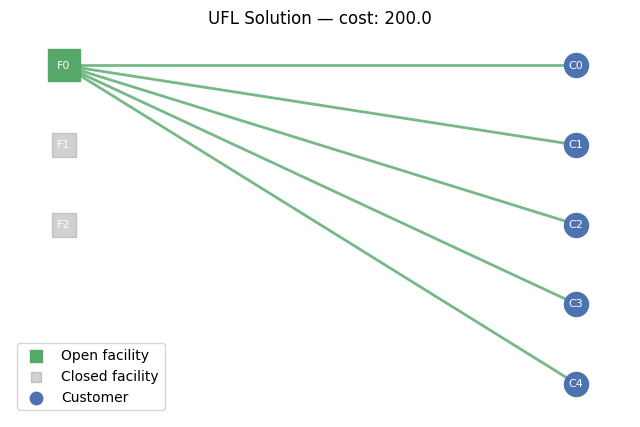
Uncapacitated Facility Location Solution:
  Open facilities: F0
  Assignments: C0 → F0, C1 → F0, C2 → F0, C3 → F0, C4 → F0
  Total cost: 200.00
    Facility cost: 100.00
    Transport cost: 100.00
  Valid: True
Plot Solution
Visualize the optimal solution showing open facilities, closed facilities, and customer assignments.
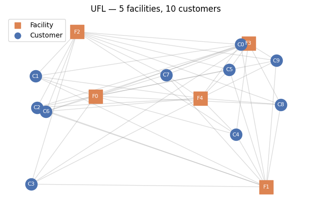
Collections
Generate a benchmark collection of random instances for batch processing.
collection = UflpCollection.from_random(
    min_num_facilities=3,
    max_num_facilities=6,
    num_instances=2,
    seed=42,
)

print(f"Collection: {collection.name}")
print(f"Description: {collection.description}")
print(f"Total instances: {len(collection.instances)}")

# Formulate the first instance
model = collection.instances[0].formulate()
print(f"\nFirst instance model: {model.name}")
Collection: Random UFL 3-6 facilities
Description: Random UFLP instances with 2 per size, customer ratio 2.0
Total instances: 8

First instance model: uncapacitated_facility_location_problem<uncapacitated_facility_location_problem>
clust = UflpCollection.from_clustered(
    min_num_facilities=3,
    max_num_facilities=6,
    cluster_std=0.15,
    seed=42,
)
clust.instances[0].data.plot()