Solving the Hamiltonian Cycle Problem

Download Notebook

In this notebook, we'll explore how to tackle the Hamiltonian Cycle problem problem using LunaSolve. First, we'll introduce and explain the Hamiltonian Cycle problem through a straightforward example. Then, we'll walk step-by-step through modeling a real-world instance, optimizing the solution, and finally interpreting the results provided by LunaSolve.

1. Hamiltonian Cycle problem

The Hamiltonian Cycle problem is a classic combinatorial optimization problem in computer science and graph theory. The problem involves determining if a given graph contains a Hamiltonian Cycle. A Hamiltonian Cycle is a route which visits every node of the graph exactly once and returns to the starting point. The possible paths which can be taken from each node are encoded by the edges connecting it to other nodes and can be directed or undirected, meaning that some paths between nodes might only be possible or more costly along a certain direction. When costs are associated with edges, the problem can become one of finding a Hamiltonian Cycle with minimal total cost which is also known as the Traveling Salesperson Problem.

Formally this means that given a graph \(G = (V, E)\) with \(V = \{ v_1, v_2, \ldots, v_n \}\) as the set of vertices and \(E\) as the set of edges. A Hamiltonian Cycle in \(G\) is a sequence of vertices \((v_{p(1)}, v_{p(2)}, \ldots, v_{p(n)})\) (where \(p(i)\) is the index of the vertex at the \(i^{th}\) position)such that :

Each vertex in \(V\) appears exactly once in the sequence.
For all \(i = 1, \ldots, n-1\), we have \((v_{p(i)}, v_{p(i+1)}) \in E\). Meaning that consecutive vertices must be connected by an edge.

2. A Real World Example

Consider this simplified scenario: A traveler wishes to plan an itinerary to visit multiple cities in a particular region. Due to limited flight availability, not all cities are directly connected by air, and the traveler can only move from one city to another if there is a flight route between them. The traveler’s goal is to determine if there exists an itinerary that allows visiting each city exactly once and then returning to the original departure city. There is no concern about flight costs or distances in this scenario—only the feasibility of such a route.

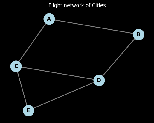
As an example, imagine we have five cities: A, B, C, D, and E. Because of limited flight routes, these cities are only sparsely connected. We can visualize this situation using a graph where each node represents a city and each edge indicates the existence of a flight connection between two cities. Some connections might be missing, which could prevent the traveler from finding a valid path that visits every city exactly once and returns to the starting point.

Vertices (Cities): U={A,B,C,D,E} Edges (Possible Routes): - (A, B) - (A, C) - (B, D) - (C, D) - (D, E)

3. Solving the Hamiltonian Cycle problem with Luna

To follow along with the next steps, you'll need the following libraries: 1. luna_usecases for modeling our optimization problem, 2. luna_quantum for solving it, 3. matplotlib for visualizing the results, and 4. networkx for creating and displaying the graphs.

Run the cell below to install these libraries automatically if they aren't already installed.

%%capture
# Install the python packages that are needed for the notebook
%pip install --upgrade pip
%pip install luna_quantum luna_usecases --upgrade
%pip install matplotlib networkx

3.1 Setting Up the Luna Client

Now let's dive into solving the Hamiltonian Cycle problem using LunaSolve. First, you'll instantiate a LunaSolve object and configure your credentials. The API key identifies your account and grants access to Luna's services. You can find your API key in your Aqarios account settings.

import os
import getpass

os.environ["LUNA_LOG_DEFAULT_LEVEL"] = "WARNING"
os.environ["LUNA_LOG_DISABLE_SPINNER"] = "true"

if "LUNA_API_KEY" not in os.environ:
    # Prompt securely for the key if not already set
    os.environ["LUNA_API_KEY"] = getpass.getpass("Enter your Luna API key: ")

from luna_quantum import LunaSolve

LunaSolve.authenticate(os.environ["LUNA_API_KEY"])
ls = LunaSolve()

If you haven't yet configured a QPU token for your account, or if you'd like to add a new one, you can do so using the ls.qpu_token.create() method. However, in this tutorial we will be using a classical solver from Dwave, which does not require one.

3.2 Create a Hamiltonian Cycle problem

Any graph with vertices and edges is enough to define a Hamiltonian Cycle problem. In this notebook, we will create a graph representing the network of flight connections between 5 cities, labeled from "A"-"E".

import matplotlib.pyplot as plt
import networkx as nx

# Define the graph
hamiltonian_cycle_graph = nx.Graph()

# Define and add the nodes of the graph. Every node represnts a city of the example.
cities = ["A", "B", "C", "D", "E"]
hamiltonian_cycle_graph.add_nodes_from(cities)

# Define and add the edges of the graph. Each edge is an available connection between cities
edges = [("A", "B"), ("A", "C"), ("B", "D"), ("C", "D"), ("D", "E"), ("E", "C")]
hamiltonian_cycle_graph.add_edges_from(edges)

# Draw the graph
pos = nx.spring_layout(hamiltonian_cycle_graph, seed=42)
nx.draw_networkx_nodes(
    hamiltonian_cycle_graph, pos, node_color="lightblue", node_size=700
)
nx.draw_networkx_labels(hamiltonian_cycle_graph, pos, font_size=12, font_weight="bold")
nx.draw_networkx_edges(hamiltonian_cycle_graph, pos, width=2, edge_color="gray")
plt.title("Flight network of Cities")
plt.axis("off")
plt.show()

png

3.3 Defining the Hamiltonian Cycle Data

The luna_usecases library ships the Hamiltonian Cycle problem as a ready-made use case. Every use case in the library follows the same five-part contract — Data, Formulation, Instance, Solution and Collection — so once you have worked through one use case, all the others work the same way.

We start with the Data class, which holds the problem instance itself.

HamiltonianCycleData describes the flight network as a binary adjacency matrix plus the matching node names. NetworkX's nx.to_numpy_array() produces exactly that matrix; passing nodelist=cities keeps its row and column order aligned with our city labels.

# Import the Hamiltonian Cycle data class from the luna_usecases library
from luna_usecases.hamiltonian_cycle import HamiltonianCycleData

# Turn the NetworkX graph into an adjacency matrix
adjacency_matrix = nx.to_numpy_array(hamiltonian_cycle_graph, nodelist=cities)

# Describe the problem instance
data = HamiltonianCycleData.from_adjacency_matrix(
    adjacency_matrix=adjacency_matrix, node_names=cities
)
print(data.to_string())

3.4 Building the Optimization Model

Next we choose a Formulation. The formulation is the recipe that turns the data into decision variables, an objective function and constraints. Printing it is a quick way to check what the resulting model will look like before it is built.

Data and formulation are then combined into an Instance, and instance.formulate() returns the optimization Model — the very same model object you would otherwise have to write by hand, ready to be handed to any Luna algorithm.

from luna_usecases.hamiltonian_cycle import (
    HamiltonianCycleFormulation,
    HamiltonianCycleInstance,
)

# Choose the formulation and inspect how the problem will be modeled
formulation = HamiltonianCycleFormulation()
print(formulation.to_string(data))

# Combine data and formulation, then build the optimization model
instance = HamiltonianCycleInstance(data=data, formulation=formulation)
model = instance.formulate()

3.5 Choose an Algorithm and Run It

The final step is to create a job request, sending our optimization task to the hardware provider to solve. In order to succesfully create a job, we must first select an algorithm for the optimization from LunaSolve's collection, specify the algorithm's parameters and select a backend for the algorithm to run on.

In this instance, we solve the Hamiltonian Cycle problem using simulated annealing (sa) and choose D-Wave (dwave) as the hardware provider. Simulated annealing has multiple parameters which can be adjusted to fine-tune the exact optimization. Here we are going to set the num_reads equal to 1000. This means that the annealing process is done 1000 times, returning 1000 sampled results.

Lastly, we exectue the job by calling the algorithm.run() method and passing the model together with a chosen namefor the job for easy identification.

from luna_quantum.algorithms import SimulatedAnnealing
from luna_quantum.backends import DWave

# Select the SimulatedAnnealingSolver algorithm.
algorithm = SimulatedAnnealing(
    backend=DWave(),
    num_reads=1000,
)

# Execute an outbound solve request.
job = algorithm.run(model, name="Hamiltonian Cycle with SA")

3.6 Retrieving the Solution

In step 3.4, we built the optimization model, and in step 3.5, we sent it to Luna to be solved. Luna automatically manages the subsequent background processes. This includes preparing the optimization problem, converting it into the correct format for the quantum hardware provider, submitting the problem to the quantum computer, and finally retrieving and translating the solution back into a user-friendly format.

Now let's discuss the final stages: retrieving the solution, converting it back to our original problem representation, and interpreting the results.

First, we'll use the job.result() method to fetch our results. The returned Solution object contains several attributes related to the optimization, including metadata such as the runtime, the count (how often each sample occurred), the objective_value and raw_energies of each sample. To learn more about the Solution Object visit Luna's thorough documentation.

solution = job.result()
print(solution)

3.7 Interpreting the Solution

The Solution object above reports the samples in the raw decision variables of the model. Reading a Hamiltonian cycle out of a table of \(x_{i,j}\) values is possible, but tedious.

This is where the Instance pays off a second time: instance.interpret() decodes a raw Solution back into the language of the use case. For the Hamiltonian Cycle problem, this returns a HamiltonianCycleSolution holding the cycle — the order in which the cities are visited — and an is_valid flag telling you whether that cycle really is a Hamiltonian cycle of our flight network.

# Decode the raw solution back into the language of the use case
hc_solution = instance.interpret(solution)
print(hc_solution.to_string())

Every use case solution can also draw itself. Passing the original problem data lets the solution highlight the result on top of the problem it belongs to.

hc_solution.plot(data)
plt.show()

Next Steps

Browse the full catalogue of ready-made problems in the use case library.
Generate whole benchmark sets of random instances with HamiltonianCycleCollection.from_random().
Swap SimulatedAnnealing for any other Luna algorithm — the model and the interpretation stay exactly the same.