Production Assignment and Scheduling (PAS) Example

Introduction

The Production Assignment and Scheduling (PAS) problem is a real-world combinatorial optimization problem that arises in manufacturing environments. The goal is to optimally assign and schedule jobs on machines while balancing three competing objectives:

Maximize job values: Each job $j$ processed on machine $m$ yields a value $v_{j,m}$, representing profit or quality
Minimize setup times: Switching between jobs on the same machine incurs setup time $s_{i,j}$ (machine-independent)
Balance machine loads: Distribute work evenly across machines to avoid bottlenecks

Problem Setting

Given: - A set of machines $\mathcal{M} = \{0, 1, 2, \ldots, M-1\}$ - A set of jobs $\mathcal{J} = \{0, 1, 2, \ldots, J-1\}$ - Processing time $p_{j,m}$ for job $j$ on machine $m$ - Setup time $s_{i,j}$ when switching from job $i$ to job $j$ - Job value $v_{j,m}$ when job $j$ is processed on machine $m$ - Eligibility constraints: Each job has a set of eligible machines $E_j \subseteq \mathcal{M}$

Mathematical Formulation

Decision Variables: $$x_{j,m,n} \in \{0, 1\}$$ where $x_{j,m,n} = 1$ if job $j$ is the $n$-th job on machine $m$, and $0$ otherwise.

Objective Function (minimization): $$\min \quad -\alpha \sum_{j,m,n} v_{j,m} \cdot x_{j,m,n} + \beta \sum_{j,j',m,n} s_{j,j'} \cdot x_{j,m,n} \cdot x_{j',m,n+1} + \gamma \sum_m \left(\sum_{j,n} p_{j,m} \cdot x_{j,m,n}\right)^2$$

where $\alpha$, $\beta$, $\gamma$ are weights for value maximization, setup minimization, and load balancing respectively.

Constraints: 1. Each job assigned exactly once: $\sum_{m,n} x_{j,m,n} = 1 \quad \forall j$ 2. At most one job per (machine, position): $\sum_j x_{j,m,n} \leq 1 \quad \forall m,n$ 3. No gaps in schedule: $\sum_j x_{j,m,n+1} \leq \sum_j x_{j,m,n} \quad \forall m,n$ 4. Eligibility: $x_{j,m,n} = 0$ if $m \notin E_j$

This notebook demonstrates how to model, solve, and analyze the PAS problem using quantum-inspired optimization.

Setup and Authentication

First, we import the necessary libraries and authenticate with the Luna Quantum SDK. The Luna platform provides access to various quantum and classical solvers for optimization problems.

import getpass
import os

from dotenv import load_dotenv

from luna_usecases.production_assignment_and_scheduling import (
    PasCollection,
    PasData,
    PasFormulation,
    PasInstance,
)

# Load environment variables from .env file
load_dotenv()

# Authenticate with Luna SDK
if "LUNA_API_KEY" not in os.environ:
    os.environ["LUNA_API_KEY"] = getpass.getpass("Enter your Luna API key: ")

api_key = os.getenv("LUNA_API_KEY")

Step 1: Create Problem Data

We generate a random PAS instance with configurable parameters. The PasData class encapsulates: - Job and machine names: Identifiers for tracking - Processing times $p_{j,m}$: Time to complete job $j$ on machine $m$ - Setup times $s_{i,j}$: Time to switch from job $i$ to job $j$ (machine-independent) - Job values $v_{j,m}$: Profit/quality when job $j$ runs on machine $m$ - Eligibility matrix: Boolean mask indicating which machines can process which jobs - Objective weights $(\alpha, \beta, \gamma)$: Trade-off parameters for the three objectives

In this example, we create a problem with 5 jobs and 2 machines, setting the balance weight to 0.5 to moderately penalize load imbalance.

data = PasData.from_random(n_jobs=5, n_machines=2, seed=42)
data.value_weight = 1.0
data.setup_weight = 1.0
data.balance_weight = 0.5
print(data.to_string())

================================================================================
PAS Data Summary
================================================================================
Jobs: 5  |  Machines: 2

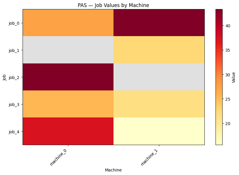
Job Values (profit/quality when job runs on machine):
------------------------------------
Job            machine_0   machine_1
------------------------------------
job_0              27.49       43.31
job_1                 --       22.49
job_2              43.29          --
job_3              25.50       21.53
job_4              37.30       15.59

Processing Times (time to complete job on machine):
------------------------------------
Job            machine_0   machine_1
------------------------------------
job_0              18.51       17.65
job_1                 --       10.10
job_2              17.68          --
job_3              17.17       16.04
job_4               7.70        6.19

Setup Times (time to switch from job i to job j):
------------------------------------------------------------------------
From \ To          job_0       job_1       job_2       job_3       job_4
------------------------------------------------------------------------
job_0               0.00        4.88        1.45        6.79        5.42
job_1               6.31        0.00        7.79        7.25        6.45
job_2               2.36        4.27        0.00        2.08        5.78
job_3               6.21        7.77        3.28        0.00        4.29
job_4               2.33        1.91        4.33        2.59        0.00

Eligibility (✓ = job can run on machine, ✗ = not allowed):
------------------------------------
Job            machine_0   machine_1
------------------------------------
job_0                  ✓           ✓
job_1                  ✗           ✓
job_2                  ✓           ✗
job_3                  ✓           ✓
job_4                  ✓           ✓

Summary Statistics:
--------------------------------------------------------------------------------
Values:           avg=   31.67  min=   15.59  max=   43.31
Processing Times: avg=   14.11  min=    6.19  max=   18.51
Setup Times:      avg=    3.74  min=    0.00  max=    7.79
Eligibility:      density= 80.0%  avg machines/job= 1.6

Objective Weights:  value=1.0  setup=1.0  balance=0.5
================================================================================

data.plot()

<Axes: title={'center': 'PAS — Job Values by Machine'}, xlabel='Machine', ylabel='Job'>

Step 2: Create the Optimization Formulation

The PasFormulation class translates the mathematical model into a constraint-based optimization problem. It: - Defines binary decision variables $x_{j,m,n}$ for each (job, machine, position) triple - Implements the four constraint types to ensure feasibility - Constructs the multi-objective function combining: - Negated value term: $-\alpha \sum v_{j,m} \cdot x_{j,m,n}$ (maximization → minimization) - Setup term: $\beta \sum s_{j,j'} \cdot x_{j,m,n} \cdot x_{j',m,n+1}$ - Balance term: $\gamma \sum_m \left(\sum p_{j,m} \cdot x_{j,m,n}\right)^2$

The formulation respects eligibility by only creating variables for valid (job, machine) pairs.

formulation = PasFormulation()
print(formulation.to_string(data))

Production Assignment and Scheduling (PAS) Formulation:
  Jobs: 5
  Machines: 2
  Max positions per machine: 5
  Eligible (job, machine) pairs: 8

Decision Variables:
  x[j,m,n] in {0,1} for eligible (j, m) pairs, n = 0, ..., 4
  x[j,m,n] = 1 if job j is the n-th job on machine m
  Total: 40 binary variables

Objective:
  minimize: -1.0×value + 1.0×setup + 0.5×balance =
  -1.0 * sum_{j,m,n} v[j,m] * x[j,m,n]
  +1.0 * sum_{j,j',m,n} s[j,j'] * x[j,m,n] * x[j',m,n+1]
  +0.5 * sum_m (sum_{j,n} p[j,m] * x[j,m,n])^2

Constraints:
  1. Each job assigned exactly once (5 constraints):
     sum_{m,n} x[j,m,n] == 1  for all j = 0, ..., 4
  2. At most one job per slot (10 constraints):
     sum_j x[j,m,n] <= 1  for all m = 0, ..., 1, n = 0, ..., 4
  3. No gaps in schedule (8 constraints):
     sum_j x[j,m,n+1] <= sum_j x[j,m,n]  for all m, n = 0, ..., 3

Step 2b: Alternative Formulation - Convex Routing Model

While the standard position-based formulation (above) uses assignment variables $x_{j,m,n}$, the convex routing formulation takes a different approach inspired by the Traveling Salesman Problem. Instead of explicitly tracking position on each machine, it uses routing variables to define the sequence of jobs as a path through a directed graph.

Key Differences from Position-Based Formulation

Aspect	Position-Based	Routing (Convex)
Variables	$x_{j,m,n}$ binary (job, machine, position)	$r_{m,i,j}$ binary (routing edges) + $c_{m,j}$ continuous (load tracking)
Sequencing	Explicit position slots $n = 0, 1, 2, \ldots$	Implicit via predecessor-successor edges
Subtour prevention	"No-gap" constraints	Capacity/MTZ-style constraints
Scalability	Variables grow as $\mathcal{O}(J \times M \times J)$	Variables grow as $\mathcal{O}(M \times J^2)$

Mathematical Formulation of Convex Routing

Decision Variables:

Routing binary variables: $r_{m,i,j} \in \{0, 1\}$
Value 1 if job $j$ directly follows job $i$ on machine $m$ (where $i$ or $j$ can be a dummy node $d = -1$ representing the start/end of the sequence)
These variables implicitly define the job sequence on each machine
Cumulative load (capacity) variables: $c_{m,j} \in \mathbb{R}_{\geq 0}$
Tracks cumulative processing time before job $j$ on machine $m$
Not in the objective — used only in constraints
Essential for preventing subtours (see constraint 5 below)
Machine total load variables: $p_m \in \mathbb{R}_{\geq 0}$
Total processing time on machine $m$ (sum of all job processing times assigned to $m$)
Appears in the objective for load balancing

Objective Weights:

$\alpha$ (value_weight): Weight for maximizing job values. Higher $\alpha$ prioritizes profit (higher values reward selecting profitable job–machine combinations)
$\beta$ (setup_weight): Weight for minimizing setup times. Higher $\beta$ discourage frequent job switches (e.g., prefer longer runs of compatible jobs)
$\gamma$ (balance_weight): Weight for load balancing. Higher $\gamma$ penalizes uneven machine utilization via the squared-load term

These are the same weights $(α, β, γ)$ as in the position-based formulation. They control the trade-off between the three competing objectives.

Objective (minimization): $$\min \quad -\alpha \sum_{m,i,j} v_{p(j),m} \cdot r_{m,i,j} + \beta \sum_{m,i,j} s_{i,j} \cdot r_{m,i,j} + \gamma \sum_{m} p_m^2$$

where: - $v_{p(j),m}$ is the value of job $j$ on machine $m$ (negated for minimization) - $s_{i,j}$ is the setup time to switch from job $i$ to job $j$ (machine-independent, same setup times as in position-based model) - $p_m^2$ is the squared load on machine $m$ (penalizes imbalance)

Constraints:

Each job has exactly one predecessor (on any eligible machine): $$\sum_{m \in E_j} \sum_{i \in \{d\} \cup J} r_{m,i,j} = 1 \quad \forall j$$
Each job has exactly one successor (on any eligible machine): $$\sum_{m \in E_j} \sum_{j' \in \{d\} \cup J} r_{m,j,j'} = 1 \quad \forall j$$
Leave dummy node at most once per machine: $$\sum_{j \in J_m} r_{m,d,j} \leq 1 \quad \forall m$$

(Ensures each machine processes at most one "chain" of jobs)

Flow conservation (including dummy node): $$\sum_{i} r_{m,i,j} = \sum_{j'} r_{m,j,j'} \quad \forall m, j \in \{d\} \cup J_m$$
Subtour elimination (Miller–Tucker–Zemlin constraints): $$c_{m,j_1} - c_{m,j_2} + M \cdot r_{m,j_1,j_2} \leq M - p_{j_2,m} \quad \forall m, j_1 \neq j_2 \in J_m$$

What this prevents: Without this constraint, the routing edges $r_{m,i,j}$ could form multiple disconnected cycles on the same machine (a "subtour"). For example, you could have jobs $\{1 \to 2 \to 1\}$ and $\{3 \to 4 \to 3\}$ on the same machine, violating the requirement that jobs form a single chain.

How it works: The variable $c_{m,j}$ tracks the cumulative processing time up to job $j$. If $r_{m,j_1,j_2} = 1$ (job $j_2$ follows $j_1$), the constraint forces $c_{m,j_1} < c_{m,j_2}$ (job $j_1$ must come before $j_2$ in time). This ordering prevents any job from appearing twice in a sequence, eliminating subtours. $M$ is a large bound (typically the sum of all processing times on a machine).

Machine load coupling: $$p_m \geq c_{m,j} \quad \forall m, j \in J_m$$
Total processing time conservation: $$\sum_m p_m = \sum_j \min_m p_{j,m}$$

(Each job must be assigned exactly once, so total load equals sum of best possible times)

Advantages of Routing Formulation

Compact representation: No explicit position variables; implicitly encoded in edges
Suitable for quantum approaches: Fewer but denser constraints (quadratic objective from setup term)
Path semantics: Naturally represents the sequence of jobs as a directed path
Better for small machines: When $M$ is small and $J$ is moderate, can be more efficient

When to Use Each Formulation

Use position-based ($PasFormulation$): Large problems with many machines, or when solver has strong support for many binary variables
Use routing ($PasConvexFormulation$): Moderate-sized problems, quantum-classical hybrid solvers, or when setup costs dominate

from luna_usecases.production_assignment_and_scheduling import PasConvexFormulation

# Create and display the convex routing formulation
convex_formulation = PasConvexFormulation()
print(convex_formulation.to_string(data))

============================================================
PAS Convex Routing Formulation
============================================================
Jobs: 5
Machines: 2
Eligible (job, machine) pairs: 8
Variables:
  r[m,i,j] = 1 if job j follows job i on machine m (i/j = d for dummy)
  c[m,j]   = cumulative load before job j on machine m
  p[m]     = total load on machine m
  Total: 50 binary routing + 8 continuous capacity + 2 continuous load

Objective:
  minimize: -1.0*value + 1.0*setup + 0.5*balance =
  -1.0 * sum_{m,pred,j} v[j,m] * r[m,pred,j]
  +1.0 * sum_{m,j,j'} s[j,j'] * r[m,j,j']
  +0.5 * sum_m p[m]^2
  where pred can be dummy d or an eligible predecessor job,
  and (j, m) / (pred, m) combinations are restricted to eligibility.

Constraints:
  1. Job predecessor/successor degree (10 constraints):
     each job has exactly one predecessor and one successor on eligible machines
     sum_{m,pred} r[m,pred,j] = 1 and sum_{m,succ} r[m,j,succ] = 1  for all jobs j
  2. Dummy departure cap (2 constraints):
     dummy can be left at most once per machine with eligible jobs
     sum_j r[m,d,j] <= 1  for all machines m with eligible jobs
  3. Self-loop elimination (10 constraints):
     disallow dummy->dummy and job->same-job arcs
     r[m,d,d] = 0 and r[m,j,j] = 0  for all machines m, jobs j
  4. Flow conservation incl. dummy (10 constraints):
     incoming flow equals outgoing flow for each node on each machine
     sum_pred r[m,pred,node] = sum_succ r[m,node,succ]  for all m, node in {d U eligible jobs}
  5. Capacity activation (8 constraints):
     c[m,j] can be positive only when job j is assigned to machine m
     c[m,j] <= M[m] * sum_pred r[m,pred,j]  for all eligible (j,m)
  6. First-job zero capacity (8 constraints):
     if dummy->j is chosen then c[m,j] must be 0
     c[m,j] <= M[m] * (1 - r[m,d,j])  for all eligible (j,m)
  7. Capacity propagation (MTZ-style) (24 constraints):
     enforce cumulative load progression along chosen arcs
     c[m,j2] >= c[m,j1] + ptime[j1,m] - M[m]*(1-r[m,j1,j2])  for j1 != j2
  8. Machine load definitions (2 constraints):
     p[m] equals total assigned processing time on machine m
     p[m] = sum_j ptime[j,m] * sum_pred r[m,pred,j]  for all machines m
  Total: 74 constraints
============================================================

Step 3: Create an Instance

The PasInstance combines the data and formulation into a single object. This design pattern allows for: - Dynamic weight overrides: You can override objective weights at the instance level without modifying the underlying data - Multiple experiments: Run the same data with different formulation parameters - Clean separation: Data (problem definition) vs. formulation (how to solve it)

The instance serves as the entry point for formulation and solution interpretation.

instance = PasInstance(data=data, formulation=formulation)
print(instance.to_string())

================================================================================
PAS Data Summary
================================================================================
Jobs: 5  |  Machines: 2

Job Values (profit/quality when job runs on machine):
------------------------------------
Job            machine_0   machine_1
------------------------------------
job_0              27.49       43.31
job_1                 --       22.49
job_2              43.29          --
job_3              25.50       21.53
job_4              37.30       15.59

Processing Times (time to complete job on machine):
------------------------------------
Job            machine_0   machine_1
------------------------------------
job_0              18.51       17.65
job_1                 --       10.10
job_2              17.68          --
job_3              17.17       16.04
job_4               7.70        6.19

Setup Times (time to switch from job i to job j):
------------------------------------------------------------------------
From \ To          job_0       job_1       job_2       job_3       job_4
------------------------------------------------------------------------
job_0               0.00        4.88        1.45        6.79        5.42
job_1               6.31        0.00        7.79        7.25        6.45
job_2               2.36        4.27        0.00        2.08        5.78
job_3               6.21        7.77        3.28        0.00        4.29
job_4               2.33        1.91        4.33        2.59        0.00

Eligibility (✓ = job can run on machine, ✗ = not allowed):
------------------------------------
Job            machine_0   machine_1
------------------------------------
job_0                  ✓           ✓
job_1                  ✗           ✓
job_2                  ✓           ✗
job_3                  ✓           ✓
job_4                  ✓           ✓

Summary Statistics:
--------------------------------------------------------------------------------
Values:           avg=   31.67  min=   15.59  max=   43.31
Processing Times: avg=   14.11  min=    6.19  max=   18.51
Setup Times:      avg=    3.74  min=    0.00  max=    7.79
Eligibility:      density= 80.0%  avg machines/job= 1.6

Objective Weights:  value=1.0  setup=1.0  balance=0.5
================================================================================
Production Assignment and Scheduling (PAS) Formulation:
  Jobs: 5
  Machines: 2
  Max positions per machine: 5
  Eligible (job, machine) pairs: 8

Decision Variables:
  x[j,m,n] in {0,1} for eligible (j, m) pairs, n = 0, ..., 4
  x[j,m,n] = 1 if job j is the n-th job on machine m
  Total: 40 binary variables

Objective:
  minimize: -1.0×value + 1.0×setup + 0.5×balance =
  -1.0 * sum_{j,m,n} v[j,m] * x[j,m,n]
  +1.0 * sum_{j,j',m,n} s[j,j'] * x[j,m,n] * x[j',m,n+1]
  +0.5 * sum_m (sum_{j,n} p[j,m] * x[j,m,n])^2

Constraints:
  1. Each job assigned exactly once (5 constraints):
     sum_{m,n} x[j,m,n] == 1  for all j = 0, ..., 4
  2. At most one job per slot (10 constraints):
     sum_j x[j,m,n] <= 1  for all m = 0, ..., 1, n = 0, ..., 4
  3. No gaps in schedule (8 constraints):
     sum_j x[j,m,n+1] <= sum_j x[j,m,n]  for all m, n = 0, ..., 3

Overriding Objective Weights

While the PasData model contains its weights ($\alpha = 1.0$, $\beta = 1.0$, $\gamma = 0.5$) that were specified at creation time, you can override these dynamically at the instance level without modifying the underlying data. This is useful for: - Parameter sensitivity analysis: Test how different weight combinations affect solutions - Multi-objective optimization: Explore the Pareto frontier by varying weight ratios - Scenario comparison: Run multiple experiments with the same data but different priorities

Simply pass value_weight, setup_weight, or balance_weight when creating the instance:

custom_instance = PasInstance(
    data=data,
    formulation=formulation,
    balance_weight=0.1  # Reduce balance penalty
)

Let's create an instance that heavily prioritizes job values while reducing the balance penalty:

# Create instance with custom weights: prioritize value, reduce balance penalty
custom_instance = PasInstance(
    data=data,
    formulation=formulation,
    value_weight=2.0,  # Double importance of job values
    balance_weight=0.1,  # Reduce balance penalty by 10x
)
print(custom_instance.to_string())

================================================================================
PAS Data Summary
================================================================================
Jobs: 5  |  Machines: 2

Job Values (profit/quality when job runs on machine):
------------------------------------
Job            machine_0   machine_1
------------------------------------
job_0              27.49       43.31
job_1                 --       22.49
job_2              43.29          --
job_3              25.50       21.53
job_4              37.30       15.59

Processing Times (time to complete job on machine):
------------------------------------
Job            machine_0   machine_1
------------------------------------
job_0              18.51       17.65
job_1                 --       10.10
job_2              17.68          --
job_3              17.17       16.04
job_4               7.70        6.19

Setup Times (time to switch from job i to job j):
------------------------------------------------------------------------
From \ To          job_0       job_1       job_2       job_3       job_4
------------------------------------------------------------------------
job_0               0.00        4.88        1.45        6.79        5.42
job_1               6.31        0.00        7.79        7.25        6.45
job_2               2.36        4.27        0.00        2.08        5.78
job_3               6.21        7.77        3.28        0.00        4.29
job_4               2.33        1.91        4.33        2.59        0.00

Eligibility (✓ = job can run on machine, ✗ = not allowed):
------------------------------------
Job            machine_0   machine_1
------------------------------------
job_0                  ✓           ✓
job_1                  ✗           ✓
job_2                  ✓           ✗
job_3                  ✓           ✓
job_4                  ✓           ✓

Summary Statistics:
--------------------------------------------------------------------------------
Values:           avg=   31.67  min=   15.59  max=   43.31
Processing Times: avg=   14.11  min=    6.19  max=   18.51
Setup Times:      avg=    3.74  min=    0.00  max=    7.79
Eligibility:      density= 80.0%  avg machines/job= 1.6

Objective Weights:  value=2.0  setup=1.0  balance=0.1
================================================================================
Production Assignment and Scheduling (PAS) Formulation:
  Jobs: 5
  Machines: 2
  Max positions per machine: 5
  Eligible (job, machine) pairs: 8

Decision Variables:
  x[j,m,n] in {0,1} for eligible (j, m) pairs, n = 0, ..., 4
  x[j,m,n] = 1 if job j is the n-th job on machine m
  Total: 40 binary variables

Objective:
  minimize: -2.0×value + 1.0×setup + 0.1×balance =
  -2.0 * sum_{j,m,n} v[j,m] * x[j,m,n]
  +1.0 * sum_{j,j',m,n} s[j,j'] * x[j,m,n] * x[j',m,n+1]
  +0.1 * sum_m (sum_{j,n} p[j,m] * x[j,m,n])^2

Constraints:
  1. Each job assigned exactly once (5 constraints):
     sum_{m,n} x[j,m,n] == 1  for all j = 0, ..., 4
  2. At most one job per slot (10 constraints):
     sum_j x[j,m,n] <= 1  for all m = 0, ..., 1, n = 0, ..., 4
  3. No gaps in schedule (8 constraints):
     sum_j x[j,m,n+1] <= sum_j x[j,m,n]  for all m, n = 0, ..., 3

Notice how the weights are reflected in the instance. When we formulate the model, these custom weights will be applied to the objective function components: - Value terms will be weighted by $\alpha = 2.0$ - Setup terms will use the default $\beta = 1.0$ - Balance terms will use the reduced $\gamma = 0.1$

# Formulate with custom weights
custom_model = custom_instance.formulate()

# Safely derive counts: handle properties, callables, or iterables
vars_obj = custom_model.variables
num_vars = getattr(custom_model, "num_variables", None)
if num_vars is None:
    num_vars = len(vars_obj() if callable(vars_obj) else vars_obj)

cons_obj = custom_model.constraints
num_cons = getattr(custom_model, "num_constraints", None)
if num_cons is None:
    num_cons = len(cons_obj() if callable(cons_obj) else cons_obj)

effective_data = custom_instance.data.model_copy(
    update={
        "value_weight": (
            custom_instance.value_weight
            if custom_instance.value_weight is not None
            else custom_instance.data.value_weight
        ),
        "setup_weight": (
            custom_instance.setup_weight
            if custom_instance.setup_weight is not None
            else custom_instance.data.setup_weight
        ),
        "balance_weight": (
            custom_instance.balance_weight
            if custom_instance.balance_weight is not None
            else custom_instance.data.balance_weight
        ),
    }
)

print(f"Custom model has {num_vars} variables and {num_cons} constraints")
print(
    f"\nData instance has original weights: alpha={custom_instance.data.value_weight},",
    f"beta={custom_instance.data.setup_weight}, gamma={custom_instance.data.balance_weight}",
)
print(
    "Objective function uses (overwritten) custom weights: "
    f"alpha={effective_data.value_weight}, "
    f"beta={effective_data.setup_weight}, gamma={effective_data.balance_weight}",
)

Custom model has 40 variables and 23 constraints

Data instance has original weights: alpha=1.0, beta=1.0, gamma=0.5
Objective function uses (overwritten) custom weights: alpha=2.0, beta=1.0, gamma=0.1

Step 4: Formulate the Quantum/Classical Model

The formulate() method generates a concrete optimization model that can be sent to various solvers. The resulting model contains: - Binary variables: One for each valid (job, machine, position) assignment - Linear constraints: Job assignment, position uniqueness, no-gap constraints - Quadratic objective: Setup terms create quadratic cross-products between consecutive positions

The model is solver-agnostic and can be executed on: - Classical MIP solvers (e.g., SCIP, Gurobi) - Quantum-classical hybrid solvers (e.g., D-Wave Hybrid, QAOA) - Quantum annealers (for small instances)

model = instance.formulate()
print(model)

Model: PAS_e30fdfce
Minimize
  342.68785494289097 * x_0_0_0 * x_0_0_1
  + 342.68785494289097 * x_0_0_0 * x_0_0_2
  + 342.68785494289097 * x_0_0_0 * x_0_0_3
  + 342.68785494289097 * x_0_0_0 * x_0_0_4
  + 327.2986450280121 * x_0_0_0 * x_2_0_0
  + 328.74536582074137 * x_0_0_0 * x_2_0_1
  + 327.2986450280121 * x_0_0_0 * x_2_0_2
  + 327.2986450280121 * x_0_0_0 * x_2_0_3
  + 327.2986450280121 * x_0_0_0 * x_2_0_4
  + 317.80333203047326 * x_0_0_0 * x_3_0_0
  + 324.59675023442134 * x_0_0_0 * x_3_0_1
  + 317.80333203047326 * x_0_0_0 * x_3_0_2
  + 317.80333203047326 * x_0_0_0 * x_3_0_3
  + 317.80333203047326 * x_0_0_0 * x_3_0_4
  + 142.60970930991263 * x_0_0_0 * x_4_0_0
  + 148.0313601037671 * x_0_0_0 * x_4_0_1
  + 142.60970930991263 * x_0_0_0 * x_4_0_2
  + 142.60970930991263 * x_0_0_0 * x_4_0_3
  + 142.60970930991263 * x_0_0_0 * x_4_0_4
  + 342.68785494289097 * x_0_0_1 * x_0_0_2
  + 342.68785494289097 * x_0_0_1 * x_0_0_3
  + 342.68785494289097 * x_0_0_1 * x_0_0_4
  + 329.6611159829759 * x_0_0_1 * x_2_0_0
  + 327.2986450280121 * x_0_0_1 * x_2_0_1
  + 328.74536582074137 * x_0_0_1 * x_2_0_2
  + 327.2986450280121 * x_0_0_1 * x_2_0_3
  + 327.2986450280121 * x_0_0_1 * x_2_0_4 + 324.016667121828 * x_0_0_1 * x_3_0_0
  + 317.80333203047326 * x_0_0_1 * x_3_0_1
  + 324.59675023442134 * x_0_0_1 * x_3_0_2
  + 317.80333203047326 * x_0_0_1 * x_3_0_3
  + 317.80333203047326 * x_0_0_1 * x_3_0_4
  + 144.93600882350262 * x_0_0_1 * x_4_0_0
  + 142.60970930991263 * x_0_0_1 * x_4_0_1
  + 148.0313601037671 * x_0_0_1 * x_4_0_2
  + 142.60970930991263 * x_0_0_1 * x_4_0_3
  + 142.60970930991263 * x_0_0_1 * x_4_0_4
  + 342.68785494289097 * x_0_0_2 * x_0_0_3
  + 342.68785494289097 * x_0_0_2 * x_0_0_4
  + 327.2986450280121 * x_0_0_2 * x_2_0_0
  + 329.6611159829759 * x_0_0_2 * x_2_0_1
  + 327.2986450280121 * x_0_0_2 * x_2_0_2
  + 328.74536582074137 * x_0_0_2 * x_2_0_3
  + 327.2986450280121 * x_0_0_2 * x_2_0_4
  + 317.80333203047326 * x_0_0_2 * x_3_0_0
  + 324.016667121828 * x_0_0_2 * x_3_0_1
  + 317.80333203047326 * x_0_0_2 * x_3_0_2
  + 324.59675023442134 * x_0_0_2 * x_3_0_3
  + 317.80333203047326 * x_0_0_2 * x_3_0_4
  + 142.60970930991263 * x_0_0_2 * x_4_0_0
  + 144.93600882350262 * x_0_0_2 * x_4_0_1
  + 142.60970930991263 * x_0_0_2 * x_4_0_2
  + 148.0313601037671 * x_0_0_2 * x_4_0_3
  + 142.60970930991263 * x_0_0_2 * x_4_0_4
  + 342.68785494289097 * x_0_0_3 * x_0_0_4
  + 327.2986450280121 * x_0_0_3 * x_2_0_0
  + 327.2986450280121 * x_0_0_3 * x_2_0_1
  + 329.6611159829759 * x_0_0_3 * x_2_0_2
  + 327.2986450280121 * x_0_0_3 * x_2_0_3
  + 328.74536582074137 * x_0_0_3 * x_2_0_4
  + 317.80333203047326 * x_0_0_3 * x_3_0_0
  + 317.80333203047326 * x_0_0_3 * x_3_0_1
  + 324.016667121828 * x_0_0_3 * x_3_0_2
  + 317.80333203047326 * x_0_0_3 * x_3_0_3
  + 324.59675023442134 * x_0_0_3 * x_3_0_4
  + 142.60970930991263 * x_0_0_3 * x_4_0_0
  + 142.60970930991263 * x_0_0_3 * x_4_0_1
  + 144.93600882350262 * x_0_0_3 * x_4_0_2
  + 142.60970930991263 * x_0_0_3 * x_4_0_3
  + 148.0313601037671 * x_0_0_3 * x_4_0_4
  + 327.2986450280121 * x_0_0_4 * x_2_0_0
  + 327.2986450280121 * x_0_0_4 * x_2_0_1
  + 327.2986450280121 * x_0_0_4 * x_2_0_2
  + 329.6611159829759 * x_0_0_4 * x_2_0_3
  + 327.2986450280121 * x_0_0_4 * x_2_0_4
  + 317.80333203047326 * x_0_0_4 * x_3_0_0
  + 317.80333203047326 * x_0_0_4 * x_3_0_1
  + 317.80333203047326 * x_0_0_4 * x_3_0_2
  + 324.016667121828 * x_0_0_4 * x_3_0_3
  + 317.80333203047326 * x_0_0_4 * x_3_0_4
  + 142.60970930991263 * x_0_0_4 * x_4_0_0
  + 142.60970930991263 * x_0_0_4 * x_4_0_1
  + 142.60970930991263 * x_0_0_4 * x_4_0_2
  + 144.93600882350262 * x_0_0_4 * x_4_0_3
  + 142.60970930991263 * x_0_0_4 * x_4_0_4
  + 311.6601688378038 * x_0_1_0 * x_0_1_1
  + 311.6601688378038 * x_0_1_0 * x_0_1_2
  + 311.6601688378038 * x_0_1_0 * x_0_1_3
  + 311.6601688378038 * x_0_1_0 * x_0_1_4
  + 178.2272576713092 * x_0_1_0 * x_1_1_0
  + 183.10935118042002 * x_0_1_0 * x_1_1_1
  + 178.2272576713092 * x_0_1_0 * x_1_1_2
  + 178.2272576713092 * x_0_1_0 * x_1_1_3
  + 178.2272576713092 * x_0_1_0 * x_1_1_4
  + 283.0975960608642 * x_0_1_0 * x_3_1_0
  + 289.89101426481227 * x_0_1_0 * x_3_1_1
  + 283.0975960608642 * x_0_1_0 * x_3_1_2
  + 283.0975960608642 * x_0_1_0 * x_3_1_3
  + 283.0975960608642 * x_0_1_0 * x_3_1_4
  + 109.21261905822807 * x_0_1_0 * x_4_1_0
  + 114.63426985208253 * x_0_1_0 * x_4_1_1
  + 109.21261905822807 * x_0_1_0 * x_4_1_2
  + 109.21261905822807 * x_0_1_0 * x_4_1_3
  + 109.21261905822807 * x_0_1_0 * x_4_1_4
  + 311.6601688378038 * x_0_1_1 * x_0_1_2
  + 311.6601688378038 * x_0_1_1 * x_0_1_3
  + 311.6601688378038 * x_0_1_1 * x_0_1_4
  + 184.5338718519068 * x_0_1_1 * x_1_1_0
  + 178.2272576713092 * x_0_1_1 * x_1_1_1
  + 183.10935118042002 * x_0_1_1 * x_1_1_2
  + 178.2272576713092 * x_0_1_1 * x_1_1_3
  + 178.2272576713092 * x_0_1_1 * x_1_1_4
  + 289.3109311522189 * x_0_1_1 * x_3_1_0
  + 283.0975960608642 * x_0_1_1 * x_3_1_1
  + 289.89101426481227 * x_0_1_1 * x_3_1_2
  + 283.0975960608642 * x_0_1_1 * x_3_1_3
  + 283.0975960608642 * x_0_1_1 * x_3_1_4
  + 111.53891857181807 * x_0_1_1 * x_4_1_0
  + 109.21261905822807 * x_0_1_1 * x_4_1_1
  + 114.63426985208253 * x_0_1_1 * x_4_1_2
  + 109.21261905822807 * x_0_1_1 * x_4_1_3
  + 109.21261905822807 * x_0_1_1 * x_4_1_4
  + 311.6601688378038 * x_0_1_2 * x_0_1_3
  + 311.6601688378038 * x_0_1_2 * x_0_1_4
  + 178.2272576713092 * x_0_1_2 * x_1_1_0
  + 184.5338718519068 * x_0_1_2 * x_1_1_1
  + 178.2272576713092 * x_0_1_2 * x_1_1_2
  + 183.10935118042002 * x_0_1_2 * x_1_1_3
  + 178.2272576713092 * x_0_1_2 * x_1_1_4
  + 283.0975960608642 * x_0_1_2 * x_3_1_0
  + 289.3109311522189 * x_0_1_2 * x_3_1_1
  + 283.0975960608642 * x_0_1_2 * x_3_1_2
  + 289.89101426481227 * x_0_1_2 * x_3_1_3
  + 283.0975960608642 * x_0_1_2 * x_3_1_4
  + 109.21261905822807 * x_0_1_2 * x_4_1_0
  + 111.53891857181807 * x_0_1_2 * x_4_1_1
  + 109.21261905822807 * x_0_1_2 * x_4_1_2
  + 114.63426985208253 * x_0_1_2 * x_4_1_3
  + 109.21261905822807 * x_0_1_2 * x_4_1_4
  + 311.6601688378038 * x_0_1_3 * x_0_1_4
  + 178.2272576713092 * x_0_1_3 * x_1_1_0
  + 178.2272576713092 * x_0_1_3 * x_1_1_1
  + 184.5338718519068 * x_0_1_3 * x_1_1_2
  + 178.2272576713092 * x_0_1_3 * x_1_1_3
  + 183.10935118042002 * x_0_1_3 * x_1_1_4
  + 283.0975960608642 * x_0_1_3 * x_3_1_0
  + 283.0975960608642 * x_0_1_3 * x_3_1_1
  + 289.3109311522189 * x_0_1_3 * x_3_1_2
  + 283.0975960608642 * x_0_1_3 * x_3_1_3
  + 289.89101426481227 * x_0_1_3 * x_3_1_4
  + 109.21261905822807 * x_0_1_3 * x_4_1_0
  + 109.21261905822807 * x_0_1_3 * x_4_1_1
  + 111.53891857181807 * x_0_1_3 * x_4_1_2
  + 109.21261905822807 * x_0_1_3 * x_4_1_3
  + 114.63426985208253 * x_0_1_3 * x_4_1_4
  + 178.2272576713092 * x_0_1_4 * x_1_1_0
  + 178.2272576713092 * x_0_1_4 * x_1_1_1
  + 178.2272576713092 * x_0_1_4 * x_1_1_2
  + 184.5338718519068 * x_0_1_4 * x_1_1_3
  + 178.2272576713092 * x_0_1_4 * x_1_1_4
  + 283.0975960608642 * x_0_1_4 * x_3_1_0
  + 283.0975960608642 * x_0_1_4 * x_3_1_1
  + 283.0975960608642 * x_0_1_4 * x_3_1_2
  + 289.3109311522189 * x_0_1_4 * x_3_1_3
  + 283.0975960608642 * x_0_1_4 * x_3_1_4
  + 109.21261905822807 * x_0_1_4 * x_4_1_0
  + 109.21261905822807 * x_0_1_4 * x_4_1_1
  + 109.21261905822807 * x_0_1_4 * x_4_1_2
  + 111.53891857181807 * x_0_1_4 * x_4_1_3
  + 109.21261905822807 * x_0_1_4 * x_4_1_4
  + 101.92176785210741 * x_1_1_0 * x_1_1_1
  + 101.92176785210741 * x_1_1_0 * x_1_1_2
  + 101.92176785210741 * x_1_1_0 * x_1_1_3
  + 101.92176785210741 * x_1_1_0 * x_1_1_4
  + 161.893348089426 * x_1_1_0 * x_3_1_0 + 169.1451959386814 * x_1_1_0 * x_3_1_1
  + 161.893348089426 * x_1_1_0 * x_3_1_2 + 161.893348089426 * x_1_1_0 * x_3_1_3
  + 161.893348089426 * x_1_1_0 * x_3_1_4
  + 62.454774604127465 * x_1_1_0 * x_4_1_0
  + 68.9034590836438 * x_1_1_0 * x_4_1_1
  + 62.454774604127465 * x_1_1_0 * x_4_1_2
  + 62.454774604127465 * x_1_1_0 * x_4_1_3
  + 62.454774604127465 * x_1_1_0 * x_4_1_4
  + 101.92176785210741 * x_1_1_1 * x_1_1_2
  + 101.92176785210741 * x_1_1_1 * x_1_1_3
  + 101.92176785210741 * x_1_1_1 * x_1_1_4
  + 169.6659162164655 * x_1_1_1 * x_3_1_0 + 161.893348089426 * x_1_1_1 * x_3_1_1
  + 169.1451959386814 * x_1_1_1 * x_3_1_2 + 161.893348089426 * x_1_1_1 * x_3_1_3
  + 161.893348089426 * x_1_1_1 * x_3_1_4 + 64.36422514147577 * x_1_1_1 * x_4_1_0
  + 62.454774604127465 * x_1_1_1 * x_4_1_1
  + 68.9034590836438 * x_1_1_1 * x_4_1_2
  + 62.454774604127465 * x_1_1_1 * x_4_1_3
  + 62.454774604127465 * x_1_1_1 * x_4_1_4
  + 101.92176785210741 * x_1_1_2 * x_1_1_3
  + 101.92176785210741 * x_1_1_2 * x_1_1_4
  + 161.893348089426 * x_1_1_2 * x_3_1_0 + 169.6659162164655 * x_1_1_2 * x_3_1_1
  + 161.893348089426 * x_1_1_2 * x_3_1_2 + 169.1451959386814 * x_1_1_2 * x_3_1_3
  + 161.893348089426 * x_1_1_2 * x_3_1_4
  + 62.454774604127465 * x_1_1_2 * x_4_1_0
  + 64.36422514147577 * x_1_1_2 * x_4_1_1
  + 62.454774604127465 * x_1_1_2 * x_4_1_2
  + 68.9034590836438 * x_1_1_2 * x_4_1_3
  + 62.454774604127465 * x_1_1_2 * x_4_1_4
  + 101.92176785210741 * x_1_1_3 * x_1_1_4
  + 161.893348089426 * x_1_1_3 * x_3_1_0 + 161.893348089426 * x_1_1_3 * x_3_1_1
  + 169.6659162164655 * x_1_1_3 * x_3_1_2 + 161.893348089426 * x_1_1_3 * x_3_1_3
  + 169.1451959386814 * x_1_1_3 * x_3_1_4
  + 62.454774604127465 * x_1_1_3 * x_4_1_0
  + 62.454774604127465 * x_1_1_3 * x_4_1_1
  + 64.36422514147577 * x_1_1_3 * x_4_1_2
  + 62.454774604127465 * x_1_1_3 * x_4_1_3
  + 68.9034590836438 * x_1_1_3 * x_4_1_4 + 161.893348089426 * x_1_1_4 * x_3_1_0
  + 161.893348089426 * x_1_1_4 * x_3_1_1 + 161.893348089426 * x_1_1_4 * x_3_1_2
  + 169.6659162164655 * x_1_1_4 * x_3_1_3 + 161.893348089426 * x_1_1_4 * x_3_1_4
  + 62.454774604127465 * x_1_1_4 * x_4_1_0
  + 62.454774604127465 * x_1_1_4 * x_4_1_1
  + 62.454774604127465 * x_1_1_4 * x_4_1_2
  + 64.36422514147577 * x_1_1_4 * x_4_1_3
  + 62.454774604127465 * x_1_1_4 * x_4_1_4
  + 312.60052403965403 * x_2_0_0 * x_2_0_1
  + 312.60052403965403 * x_2_0_0 * x_2_0_2
  + 312.60052403965403 * x_2_0_0 * x_2_0_3
  + 312.60052403965403 * x_2_0_0 * x_2_0_4
  + 303.5316205655895 * x_2_0_0 * x_3_0_0
  + 305.6116470100623 * x_2_0_0 * x_3_0_1
  + 303.5316205655895 * x_2_0_0 * x_3_0_2
  + 303.5316205655895 * x_2_0_0 * x_3_0_3
  + 303.5316205655895 * x_2_0_0 * x_3_0_4
  + 136.20548248712126 * x_2_0_0 * x_4_0_0
  + 141.98682515981844 * x_2_0_0 * x_4_0_1
  + 136.20548248712126 * x_2_0_0 * x_4_0_2
  + 136.20548248712126 * x_2_0_0 * x_4_0_3
  + 136.20548248712126 * x_2_0_0 * x_4_0_4
  + 312.60052403965403 * x_2_0_1 * x_2_0_2
  + 312.60052403965403 * x_2_0_1 * x_2_0_3
  + 312.60052403965403 * x_2_0_1 * x_2_0_4
  + 306.81239807255656 * x_2_0_1 * x_3_0_0
  + 303.5316205655895 * x_2_0_1 * x_3_0_1
  + 305.6116470100623 * x_2_0_1 * x_3_0_2
  + 303.5316205655895 * x_2_0_1 * x_3_0_3
  + 303.5316205655895 * x_2_0_1 * x_3_0_4
  + 140.53541697070278 * x_2_0_1 * x_4_0_0
  + 136.20548248712126 * x_2_0_1 * x_4_0_1
  + 141.98682515981844 * x_2_0_1 * x_4_0_2
  + 136.20548248712126 * x_2_0_1 * x_4_0_3
  + 136.20548248712126 * x_2_0_1 * x_4_0_4
  + 312.60052403965403 * x_2_0_2 * x_2_0_3
  + 312.60052403965403 * x_2_0_2 * x_2_0_4
  + 303.5316205655895 * x_2_0_2 * x_3_0_0
  + 306.81239807255656 * x_2_0_2 * x_3_0_1
  + 303.5316205655895 * x_2_0_2 * x_3_0_2
  + 305.6116470100623 * x_2_0_2 * x_3_0_3
  + 303.5316205655895 * x_2_0_2 * x_3_0_4
  + 136.20548248712126 * x_2_0_2 * x_4_0_0
  + 140.53541697070278 * x_2_0_2 * x_4_0_1
  + 136.20548248712126 * x_2_0_2 * x_4_0_2
  + 141.98682515981844 * x_2_0_2 * x_4_0_3
  + 136.20548248712126 * x_2_0_2 * x_4_0_4
  + 312.60052403965403 * x_2_0_3 * x_2_0_4
  + 303.5316205655895 * x_2_0_3 * x_3_0_0
  + 303.5316205655895 * x_2_0_3 * x_3_0_1
  + 306.81239807255656 * x_2_0_3 * x_3_0_2
  + 303.5316205655895 * x_2_0_3 * x_3_0_3
  + 305.6116470100623 * x_2_0_3 * x_3_0_4
  + 136.20548248712126 * x_2_0_3 * x_4_0_0
  + 136.20548248712126 * x_2_0_3 * x_4_0_1
  + 140.53541697070278 * x_2_0_3 * x_4_0_2
  + 136.20548248712126 * x_2_0_3 * x_4_0_3
  + 141.98682515981844 * x_2_0_3 * x_4_0_4
  + 303.5316205655895 * x_2_0_4 * x_3_0_0
  + 303.5316205655895 * x_2_0_4 * x_3_0_1
  + 303.5316205655895 * x_2_0_4 * x_3_0_2
  + 306.81239807255656 * x_2_0_4 * x_3_0_3
  + 303.5316205655895 * x_2_0_4 * x_3_0_4
  + 136.20548248712126 * x_2_0_4 * x_4_0_0
  + 136.20548248712126 * x_2_0_4 * x_4_0_1
  + 136.20548248712126 * x_2_0_4 * x_4_0_2
  + 140.53541697070278 * x_2_0_4 * x_4_0_3
  + 136.20548248712126 * x_2_0_4 * x_4_0_4
  + 294.7258164912286 * x_3_0_0 * x_3_0_1
  + 294.7258164912286 * x_3_0_0 * x_3_0_2
  + 294.7258164912286 * x_3_0_0 * x_3_0_3
  + 294.7258164912286 * x_3_0_0 * x_3_0_4
  + 132.25400359210377 * x_3_0_0 * x_4_0_0
  + 136.54089427103443 * x_3_0_0 * x_4_0_1
  + 132.25400359210377 * x_3_0_0 * x_4_0_2
  + 132.25400359210377 * x_3_0_0 * x_4_0_3
  + 132.25400359210377 * x_3_0_0 * x_4_0_4
  + 294.7258164912286 * x_3_0_1 * x_3_0_2
  + 294.7258164912286 * x_3_0_1 * x_3_0_3
  + 294.7258164912286 * x_3_0_1 * x_3_0_4
  + 134.84236903545997 * x_3_0_1 * x_4_0_0
  + 132.25400359210377 * x_3_0_1 * x_4_0_1
  + 136.54089427103443 * x_3_0_1 * x_4_0_2
  + 132.25400359210377 * x_3_0_1 * x_4_0_3
  + 132.25400359210377 * x_3_0_1 * x_4_0_4
  + 294.7258164912286 * x_3_0_2 * x_3_0_3
  + 294.7258164912286 * x_3_0_2 * x_3_0_4
  + 132.25400359210377 * x_3_0_2 * x_4_0_0
  + 134.84236903545997 * x_3_0_2 * x_4_0_1
  + 132.25400359210377 * x_3_0_2 * x_4_0_2
  + 136.54089427103443 * x_3_0_2 * x_4_0_3
  + 132.25400359210377 * x_3_0_2 * x_4_0_4
  + 294.7258164912286 * x_3_0_3 * x_3_0_4
  + 132.25400359210377 * x_3_0_3 * x_4_0_0
  + 132.25400359210377 * x_3_0_3 * x_4_0_1
  + 134.84236903545997 * x_3_0_3 * x_4_0_2
  + 132.25400359210377 * x_3_0_3 * x_4_0_3
  + 136.54089427103443 * x_3_0_3 * x_4_0_4
  + 132.25400359210377 * x_3_0_4 * x_4_0_0
  + 132.25400359210377 * x_3_0_4 * x_4_0_1
  + 132.25400359210377 * x_3_0_4 * x_4_0_2
  + 134.84236903545997 * x_3_0_4 * x_4_0_3
  + 132.25400359210377 * x_3_0_4 * x_4_0_4
  + 257.15268394515124 * x_3_1_0 * x_3_1_1
  + 257.15268394515124 * x_3_1_0 * x_3_1_2
  + 257.15268394515124 * x_3_1_0 * x_3_1_3
  + 257.15268394515124 * x_3_1_0 * x_3_1_4
  + 99.20366157212007 * x_3_1_0 * x_4_1_0
  + 103.49055225105073 * x_3_1_0 * x_4_1_1
  + 99.20366157212007 * x_3_1_0 * x_4_1_2
  + 99.20366157212007 * x_3_1_0 * x_4_1_3
  + 99.20366157212007 * x_3_1_0 * x_4_1_4
  + 257.15268394515124 * x_3_1_1 * x_3_1_2
  + 257.15268394515124 * x_3_1_1 * x_3_1_3
  + 257.15268394515124 * x_3_1_1 * x_3_1_4
  + 101.79202701547626 * x_3_1_1 * x_4_1_0
  + 99.20366157212007 * x_3_1_1 * x_4_1_1
  + 103.49055225105073 * x_3_1_1 * x_4_1_2
  + 99.20366157212007 * x_3_1_1 * x_4_1_3
  + 99.20366157212007 * x_3_1_1 * x_4_1_4
  + 257.15268394515124 * x_3_1_2 * x_3_1_3
  + 257.15268394515124 * x_3_1_2 * x_3_1_4
  + 99.20366157212007 * x_3_1_2 * x_4_1_0
  + 101.79202701547626 * x_3_1_2 * x_4_1_1
  + 99.20366157212007 * x_3_1_2 * x_4_1_2
  + 103.49055225105073 * x_3_1_2 * x_4_1_3
  + 99.20366157212007 * x_3_1_2 * x_4_1_4
  + 257.15268394515124 * x_3_1_3 * x_3_1_4
  + 99.20366157212007 * x_3_1_3 * x_4_1_0
  + 99.20366157212007 * x_3_1_3 * x_4_1_1
  + 101.79202701547626 * x_3_1_3 * x_4_1_2
  + 99.20366157212007 * x_3_1_3 * x_4_1_3
  + 103.49055225105073 * x_3_1_3 * x_4_1_4
  + 99.20366157212007 * x_3_1_4 * x_4_1_0
  + 99.20366157212007 * x_3_1_4 * x_4_1_1
  + 99.20366157212007 * x_3_1_4 * x_4_1_2
  + 101.79202701547626 * x_3_1_4 * x_4_1_3
  + 99.20366157212007 * x_3_1_4 * x_4_1_4
  + 59.34709647894302 * x_4_0_0 * x_4_0_1
  + 59.34709647894302 * x_4_0_0 * x_4_0_2
  + 59.34709647894302 * x_4_0_0 * x_4_0_3
  + 59.34709647894302 * x_4_0_0 * x_4_0_4
  + 59.34709647894302 * x_4_0_1 * x_4_0_2
  + 59.34709647894302 * x_4_0_1 * x_4_0_3
  + 59.34709647894302 * x_4_0_1 * x_4_0_4
  + 59.34709647894302 * x_4_0_2 * x_4_0_3
  + 59.34709647894302 * x_4_0_2 * x_4_0_4
  + 59.34709647894302 * x_4_0_3 * x_4_0_4
  + 38.270518193054606 * x_4_1_0 * x_4_1_1
  + 38.270518193054606 * x_4_1_0 * x_4_1_2
  + 38.270518193054606 * x_4_1_0 * x_4_1_3
  + 38.270518193054606 * x_4_1_0 * x_4_1_4
  + 38.270518193054606 * x_4_1_1 * x_4_1_2
  + 38.270518193054606 * x_4_1_1 * x_4_1_3
  + 38.270518193054606 * x_4_1_1 * x_4_1_4
  + 38.270518193054606 * x_4_1_2 * x_4_1_3
  + 38.270518193054606 * x_4_1_2 * x_4_1_4
  + 38.270518193054606 * x_4_1_3 * x_4_1_4 + 143.85785071655226 * x_0_0_0
  + 143.85785071655226 * x_0_0_1 + 143.85785071655226 * x_0_0_2
  + 143.85785071655226 * x_0_0_3 + 143.85785071655226 * x_0_0_4
  + 112.5229565765884 * x_0_1_0 + 112.5229565765884 * x_0_1_1
  + 112.5229565765884 * x_0_1_2 + 112.5229565765884 * x_0_1_3
  + 112.5229565765884 * x_0_1_4 + 28.46621827077206 * x_1_1_0
  + 28.46621827077206 * x_1_1_1 + 28.46621827077206 * x_1_1_2
  + 28.46621827077206 * x_1_1_3 + 28.46621827077206 * x_1_1_4
  + 113.00986996401897 * x_2_0_0 + 113.00986996401897 * x_2_0_1
  + 113.00986996401897 * x_2_0_2 + 113.00986996401897 * x_2_0_3
  + 113.00986996401897 * x_2_0_4 + 121.86377308440733 * x_3_0_0
  + 121.86377308440733 * x_3_0_1 + 121.86377308440733 * x_3_0_2
  + 121.86377308440733 * x_3_0_3 + 121.86377308440733 * x_3_0_4
  + 107.04321781536586 * x_3_1_0 + 107.04321781536586 * x_3_1_1
  + 107.04321781536586 * x_3_1_2 + 107.04321781536586 * x_3_1_3
  + 107.04321781536586 * x_3_1_4 - 7.6262719195275075 * x_4_0_0
  - 7.6262719195275075 * x_4_0_1 - 7.6262719195275075 * x_4_0_2
  - 7.6262719195275075 * x_4_0_3 - 7.6262719195275075 * x_4_0_4
  + 3.5451597521549107 * x_4_1_0 + 3.5451597521549107 * x_4_1_1
  + 3.5451597521549107 * x_4_1_2 + 3.5451597521549107 * x_4_1_3
  + 3.5451597521549107 * x_4_1_4
Subject To
  job_0_assigned_once: x_0_0_0 + x_0_0_1 + x_0_0_2 + x_0_0_3 + x_0_0_4 + x_0_1_0
    + x_0_1_1 + x_0_1_2 + x_0_1_3 + x_0_1_4 == 1
  job_1_assigned_once: x_1_1_0 + x_1_1_1 + x_1_1_2 + x_1_1_3 + x_1_1_4 == 1
  job_2_assigned_once: x_2_0_0 + x_2_0_1 + x_2_0_2 + x_2_0_3 + x_2_0_4 == 1
  job_3_assigned_once: x_3_0_0 + x_3_0_1 + x_3_0_2 + x_3_0_3 + x_3_0_4 + x_3_1_0
    + x_3_1_1 + x_3_1_2 + x_3_1_3 + x_3_1_4 == 1
  job_4_assigned_once: x_4_0_0 + x_4_0_1 + x_4_0_2 + x_4_0_3 + x_4_0_4 + x_4_1_0
    + x_4_1_1 + x_4_1_2 + x_4_1_3 + x_4_1_4 == 1
  machine_0_position_0_max_one_job: x_0_0_0 + x_2_0_0 + x_3_0_0 + x_4_0_0 <= 1
  machine_0_position_1_max_one_job: x_0_0_1 + x_2_0_1 + x_3_0_1 + x_4_0_1 <= 1
  machine_0_position_2_max_one_job: x_0_0_2 + x_2_0_2 + x_3_0_2 + x_4_0_2 <= 1
  machine_0_position_3_max_one_job: x_0_0_3 + x_2_0_3 + x_3_0_3 + x_4_0_3 <= 1
  machine_0_position_4_max_one_job: x_0_0_4 + x_2_0_4 + x_3_0_4 + x_4_0_4 <= 1
  machine_1_position_0_max_one_job: x_0_1_0 + x_1_1_0 + x_3_1_0 + x_4_1_0 <= 1
  machine_1_position_1_max_one_job: x_0_1_1 + x_1_1_1 + x_3_1_1 + x_4_1_1 <= 1
  machine_1_position_2_max_one_job: x_0_1_2 + x_1_1_2 + x_3_1_2 + x_4_1_2 <= 1
  machine_1_position_3_max_one_job: x_0_1_3 + x_1_1_3 + x_3_1_3 + x_4_1_3 <= 1
  machine_1_position_4_max_one_job: x_0_1_4 + x_1_1_4 + x_3_1_4 + x_4_1_4 <= 1
  machine_0_no_gap_at_0: -x_0_0_0 + x_0_0_1 - x_2_0_0 + x_2_0_1 - x_3_0_0
    + x_3_0_1 - x_4_0_0 + x_4_0_1 <= 0
  machine_0_no_gap_at_1: -x_0_0_1 + x_0_0_2 - x_2_0_1 + x_2_0_2 - x_3_0_1
    + x_3_0_2 - x_4_0_1 + x_4_0_2 <= 0
  machine_0_no_gap_at_2: -x_0_0_2 + x_0_0_3 - x_2_0_2 + x_2_0_3 - x_3_0_2
    + x_3_0_3 - x_4_0_2 + x_4_0_3 <= 0
  machine_0_no_gap_at_3: -x_0_0_3 + x_0_0_4 - x_2_0_3 + x_2_0_4 - x_3_0_3
    + x_3_0_4 - x_4_0_3 + x_4_0_4 <= 0
  machine_1_no_gap_at_0: -x_0_1_0 + x_0_1_1 - x_1_1_0 + x_1_1_1 - x_3_1_0
    + x_3_1_1 - x_4_1_0 + x_4_1_1 <= 0
  machine_1_no_gap_at_1: -x_0_1_1 + x_0_1_2 - x_1_1_1 + x_1_1_2 - x_3_1_1
    + x_3_1_2 - x_4_1_1 + x_4_1_2 <= 0
  machine_1_no_gap_at_2: -x_0_1_2 + x_0_1_3 - x_1_1_2 + x_1_1_3 - x_3_1_2
    + x_3_1_3 - x_4_1_2 + x_4_1_3 <= 0
  machine_1_no_gap_at_3: -x_0_1_3 + x_0_1_4 - x_1_1_3 + x_1_1_4 - x_3_1_3
    + x_3_1_4 - x_4_1_3 + x_4_1_4 <= 0
Binary
  x_0_0_0 x_0_0_1 x_0_0_2 x_0_0_3 x_0_0_4 x_0_1_0 x_0_1_1 x_0_1_2 x_0_1_3
  x_0_1_4 x_1_1_0 x_1_1_1 x_1_1_2 x_1_1_3 x_1_1_4 x_2_0_0 x_2_0_1 x_2_0_2
  x_2_0_3 x_2_0_4 x_3_0_0 x_3_0_1 x_3_0_2 x_3_0_3 x_3_0_4 x_3_1_0 x_3_1_1
  x_3_1_2 x_3_1_3 x_3_1_4 x_4_0_0 x_4_0_1 x_4_0_2 x_4_0_3 x_4_0_4 x_4_1_0
  x_4_1_1 x_4_1_2 x_4_1_3 x_4_1_4

Convex Routing Model Instance

Now let's create an instance with the convex formulation for comparison:

convex_instance = PasInstance(data=data, formulation=convex_formulation)
convex_model = convex_instance.formulate()
print("\n=== CONVEX ROUTING MODEL INSTANCE ===\n")
print(convex_model)

=== CONVEX ROUTING MODEL INSTANCE ===

Model: PAS_CONVEX_e30fdfce
Minimize
  0.5 * p_0 * p_0 + 0.5 * p_1 * p_1 - 27.48607675489323 * r_0_d_0
  - 43.29039205580804 * r_0_d_2 - 25.49913516120698 * r_0_d_3
  - 37.29982015899902 * r_0_d_4 - 27.48607675489323 * r_0_0_0
  - 41.84367126307882 * r_0_0_2 - 18.705716957258904 * r_0_0_3
  - 31.878169365144565 * r_0_0_4 - 25.123605799929457 * r_0_2_0
  - 43.29039205580804 * r_0_2_2 - 23.419108716734144 * r_0_2_3
  - 31.518477486301837 * r_0_2_4 - 21.27274166353851 * r_0_3_0
  - 40.00961454884098 * r_0_3_2 - 25.49913516120698 * r_0_3_3
  - 33.012929480068365 * r_0_3_4 - 25.159777241303228 * r_0_4_0
  - 38.9604575722265 * r_0_4_2 - 22.91076971785079 * r_0_4_3
  - 37.29982015899902 * r_0_4_4 - 43.3071278423135 * r_1_d_0
  - 22.494665655281644 * r_1_d_1 - 21.533124157209762 * r_1_d_3
  - 15.590099344372392 * r_1_d_4 - 43.3071278423135 * r_1_0_0
  - 17.6125721461708 * r_1_0_1 - 14.739705953261687 * r_1_0_3
  - 10.168448550517939 * r_1_0_4 - 37.000513661715885 * r_1_1_0
  - 22.494665655281644 * r_1_1_1 - 14.281276307954379 * r_1_1_3
  - 9.14141486485606 * r_1_1_4 - 37.09379275095878 * r_1_3_0
  - 14.722097528242173 * r_1_3_1 - 21.533124157209762 * r_1_3_3
  - 11.303208665441737 * r_1_3_4 - 40.9808283287235 * r_1_4_0
  - 20.58521511793334 * r_1_4_1 - 18.944758713853574 * r_1_4_3
  - 15.590099344372392 * r_1_4_4
Subject To
  job_0_one_successor: r_0_0_d + r_0_0_0 + r_0_0_2 + r_0_0_3 + r_0_0_4 + r_1_0_d
    + r_1_0_0 + r_1_0_1 + r_1_0_3 + r_1_0_4 == 1
  job_1_one_successor: r_1_1_d + r_1_1_0 + r_1_1_1 + r_1_1_3 + r_1_1_4 == 1
  job_2_one_successor: r_0_2_d + r_0_2_0 + r_0_2_2 + r_0_2_3 + r_0_2_4 == 1
  job_3_one_successor: r_0_3_d + r_0_3_0 + r_0_3_2 + r_0_3_3 + r_0_3_4 + r_1_3_d
    + r_1_3_0 + r_1_3_1 + r_1_3_3 + r_1_3_4 == 1
  job_4_one_successor: r_0_4_d + r_0_4_0 + r_0_4_2 + r_0_4_3 + r_0_4_4 + r_1_4_d
    + r_1_4_0 + r_1_4_1 + r_1_4_3 + r_1_4_4 == 1
  job_0_one_predecessor: r_0_d_0 + r_0_0_0 + r_0_2_0 + r_0_3_0 + r_0_4_0
    + r_1_d_0 + r_1_0_0 + r_1_1_0 + r_1_3_0 + r_1_4_0 == 1
  job_1_one_predecessor: r_1_d_1 + r_1_0_1 + r_1_1_1 + r_1_3_1 + r_1_4_1 == 1
  job_2_one_predecessor: r_0_d_2 + r_0_0_2 + r_0_2_2 + r_0_3_2 + r_0_4_2 == 1
  job_3_one_predecessor: r_0_d_3 + r_0_0_3 + r_0_2_3 + r_0_3_3 + r_0_4_3
    + r_1_d_3 + r_1_0_3 + r_1_1_3 + r_1_3_3 + r_1_4_3 == 1
  job_4_one_predecessor: r_0_d_4 + r_0_0_4 + r_0_2_4 + r_0_3_4 + r_0_4_4
    + r_1_d_4 + r_1_0_4 + r_1_1_4 + r_1_3_4 + r_1_4_4 == 1
  machine_0_leave_dummy_once: r_0_d_0 + r_0_d_2 + r_0_d_3 + r_0_d_4 <= 1
  machine_1_leave_dummy_once: r_1_d_0 + r_1_d_1 + r_1_d_3 + r_1_d_4 <= 1
  machine_0_no_dummy_self_loop: r_0_d_d == 0
  machine_0_no_job_self_loop_0: r_0_0_0 == 0
  machine_0_no_job_self_loop_2: r_0_2_2 == 0
  machine_0_no_job_self_loop_3: r_0_3_3 == 0
  machine_0_no_job_self_loop_4: r_0_4_4 == 0
  machine_1_no_dummy_self_loop: r_1_d_d == 0
  machine_1_no_job_self_loop_0: r_1_0_0 == 0
  machine_1_no_job_self_loop_1: r_1_1_1 == 0
  machine_1_no_job_self_loop_3: r_1_3_3 == 0
  machine_1_no_job_self_loop_4: r_1_4_4 == 0
  machine_0_flow_d: -r_0_d_0 - r_0_d_2 - r_0_d_3 - r_0_d_4 + r_0_0_d + r_0_2_d
    + r_0_3_d + r_0_4_d == 0
  machine_0_flow_0: r_0_d_0 - r_0_0_d - r_0_0_2 - r_0_0_3 - r_0_0_4 + r_0_2_0
    + r_0_3_0 + r_0_4_0 == 0
  machine_0_flow_2: r_0_d_2 + r_0_0_2 - r_0_2_d - r_0_2_0 - r_0_2_3 - r_0_2_4
    + r_0_3_2 + r_0_4_2 == 0
  machine_0_flow_3: r_0_d_3 + r_0_0_3 + r_0_2_3 - r_0_3_d - r_0_3_0 - r_0_3_2
    - r_0_3_4 + r_0_4_3 == 0
  machine_0_flow_4: r_0_d_4 + r_0_0_4 + r_0_2_4 + r_0_3_4 - r_0_4_d - r_0_4_0
    - r_0_4_2 - r_0_4_3 == 0
  machine_1_flow_d: -r_1_d_0 - r_1_d_1 - r_1_d_3 - r_1_d_4 + r_1_0_d + r_1_1_d
    + r_1_3_d + r_1_4_d == 0
  machine_1_flow_0: r_1_d_0 - r_1_0_d - r_1_0_1 - r_1_0_3 - r_1_0_4 + r_1_1_0
    + r_1_3_0 + r_1_4_0 == 0
  machine_1_flow_1: r_1_d_1 + r_1_0_1 - r_1_1_d - r_1_1_0 - r_1_1_3 - r_1_1_4
    + r_1_3_1 + r_1_4_1 == 0
  machine_1_flow_3: r_1_d_3 + r_1_0_3 + r_1_1_3 - r_1_3_d - r_1_3_0 - r_1_3_1
    - r_1_3_4 + r_1_4_3 == 0
  machine_1_flow_4: r_1_d_4 + r_1_0_4 + r_1_1_4 + r_1_3_4 - r_1_4_d - r_1_4_0
    - r_1_4_1 - r_1_4_3 == 0
  machine_0_capacity_active_0: -61.063629747822404 * r_0_d_0
    - 61.063629747822404 * r_0_0_0 - 61.063629747822404 * r_0_2_0
    - 61.063629747822404 * r_0_3_0 - 61.063629747822404 * r_0_4_0 + c_0_0 <= 0
  machine_0_first_job_zero_capacity_0: 61.063629747822404 * r_0_d_0 + c_0_0 <=
    61.063629747822404
  machine_0_capacity_active_2: -61.063629747822404 * r_0_d_2
    - 61.063629747822404 * r_0_0_2 - 61.063629747822404 * r_0_2_2
    - 61.063629747822404 * r_0_3_2 - 61.063629747822404 * r_0_4_2 + c_0_2 <= 0
  machine_0_first_job_zero_capacity_2: 61.063629747822404 * r_0_d_2 + c_0_2 <=
    61.063629747822404
  machine_0_capacity_active_3: -61.063629747822404 * r_0_d_3
    - 61.063629747822404 * r_0_0_3 - 61.063629747822404 * r_0_2_3
    - 61.063629747822404 * r_0_3_3 - 61.063629747822404 * r_0_4_3 + c_0_3 <= 0
  machine_0_first_job_zero_capacity_3: 61.063629747822404 * r_0_d_3 + c_0_3 <=
    61.063629747822404
  machine_0_capacity_active_4: -61.063629747822404 * r_0_d_4
    - 61.063629747822404 * r_0_0_4 - 61.063629747822404 * r_0_2_4
    - 61.063629747822404 * r_0_3_4 - 61.063629747822404 * r_0_4_4 + c_0_4 <= 0
  machine_0_first_job_zero_capacity_4: 61.063629747822404 * r_0_d_4 + c_0_4 <=
    61.063629747822404
  machine_0_capacity_propagation_0_2: -61.063629747822404 * r_0_0_2 - c_0_0
    + c_0_2 >= -42.55179961293593
  machine_0_capacity_propagation_0_3: -61.063629747822404 * r_0_0_3 - c_0_0
    + c_0_3 >= -42.55179961293593
  machine_0_capacity_propagation_0_4: -61.063629747822404 * r_0_0_4 - c_0_0
    + c_0_4 >= -42.55179961293593
  machine_0_capacity_propagation_2_0: -61.063629747822404 * r_0_2_0 + c_0_0
    - c_0_2 >= -43.3831171975694
  machine_0_capacity_propagation_2_3: -61.063629747822404 * r_0_2_3 - c_0_2
    + c_0_3 >= -43.3831171975694
  machine_0_capacity_propagation_2_4: -61.063629747822404 * r_0_2_4 - c_0_2
    + c_0_4 >= -43.3831171975694
  machine_0_capacity_propagation_3_0: -61.063629747822404 * r_0_3_0 + c_0_0
    - c_0_3 >= -43.89604935653754
  machine_0_capacity_propagation_3_2: -61.063629747822404 * r_0_3_2 + c_0_2
    - c_0_3 >= -43.89604935653754
  machine_0_capacity_propagation_3_4: -61.063629747822404 * r_0_3_4 - c_0_3
    + c_0_4 >= -43.89604935653754
  machine_0_capacity_propagation_4_0: -61.063629747822404 * r_0_4_0 + c_0_0
    - c_0_4 >= -53.35992307642434
  machine_0_capacity_propagation_4_2: -61.063629747822404 * r_0_4_2 + c_0_2
    - c_0_4 >= -53.35992307642434
  machine_0_capacity_propagation_4_3: -61.063629747822404 * r_0_4_3 + c_0_3
    - c_0_4 >= -53.35992307642434
  machine_1_capacity_active_0: -49.97182859312102 * r_1_d_0
    - 49.97182859312102 * r_1_0_0 - 49.97182859312102 * r_1_1_0
    - 49.97182859312102 * r_1_3_0 - 49.97182859312102 * r_1_4_0 + c_1_0 <= 0
  machine_1_first_job_zero_capacity_0: 49.97182859312102 * r_1_d_0 + c_1_0 <=
    49.97182859312102
  machine_1_capacity_active_1: -49.97182859312102 * r_1_d_1
    - 49.97182859312102 * r_1_0_1 - 49.97182859312102 * r_1_1_1
    - 49.97182859312102 * r_1_3_1 - 49.97182859312102 * r_1_4_1 + c_1_1 <= 0
  machine_1_first_job_zero_capacity_1: 49.97182859312102 * r_1_d_1 + c_1_1 <=
    49.97182859312102
  machine_1_capacity_active_3: -49.97182859312102 * r_1_d_3
    - 49.97182859312102 * r_1_0_3 - 49.97182859312102 * r_1_1_3
    - 49.97182859312102 * r_1_3_3 - 49.97182859312102 * r_1_4_3 + c_1_3 <= 0
  machine_1_first_job_zero_capacity_3: 49.97182859312102 * r_1_d_3 + c_1_3 <=
    49.97182859312102
  machine_1_capacity_active_4: -49.97182859312102 * r_1_d_4
    - 49.97182859312102 * r_1_0_4 - 49.97182859312102 * r_1_1_4
    - 49.97182859312102 * r_1_3_4 - 49.97182859312102 * r_1_4_4 + c_1_4 <= 0
  machine_1_first_job_zero_capacity_4: 49.97182859312102 * r_1_d_4 + c_1_4 <=
    49.97182859312102
  machine_1_capacity_propagation_0_1: -49.97182859312102 * r_1_0_1 - c_1_0
    + c_1_1 >= -32.317929056820155
  machine_1_capacity_propagation_0_3: -49.97182859312102 * r_1_0_3 - c_1_0
    + c_1_3 >= -32.317929056820155
  machine_1_capacity_propagation_0_4: -49.97182859312102 * r_1_0_4 - c_1_0
    + c_1_4 >= -32.317929056820155
  machine_1_capacity_propagation_1_0: -49.97182859312102 * r_1_1_0 + c_1_0
    - c_1_1 >= -39.87619746613805
  machine_1_capacity_propagation_1_3: -49.97182859312102 * r_1_1_3 - c_1_1
    + c_1_3 >= -39.87619746613805
  machine_1_capacity_propagation_1_4: -49.97182859312102 * r_1_1_4 - c_1_1
    + c_1_4 >= -39.87619746613805
  machine_1_capacity_propagation_3_0: -49.97182859312102 * r_1_3_0 + c_1_0
    - c_1_3 >= -33.9358476769079
  machine_1_capacity_propagation_3_1: -49.97182859312102 * r_1_3_1 + c_1_1
    - c_1_3 >= -33.9358476769079
  machine_1_capacity_propagation_3_4: -49.97182859312102 * r_1_3_4 - c_1_3
    + c_1_4 >= -33.9358476769079
  machine_1_capacity_propagation_4_0: -49.97182859312102 * r_1_4_0 + c_1_0
    - c_1_4 >= -43.78551157949695
  machine_1_capacity_propagation_4_1: -49.97182859312102 * r_1_4_1 + c_1_1
    - c_1_4 >= -43.78551157949695
  machine_1_capacity_propagation_4_3: -49.97182859312102 * r_1_4_3 + c_1_3
    - c_1_4 >= -43.78551157949695
  machine_0_ptime_definition: -18.511830134886473 * r_0_d_0
    - 17.680512550253006 * r_0_d_2 - 17.167580391284865 * r_0_d_3
    - 7.703706671398063 * r_0_d_4 - 18.511830134886473 * r_0_0_0
    - 17.680512550253006 * r_0_0_2 - 17.167580391284865 * r_0_0_3
    - 7.703706671398063 * r_0_0_4 - 18.511830134886473 * r_0_2_0
    - 17.680512550253006 * r_0_2_2 - 17.167580391284865 * r_0_2_3
    - 7.703706671398063 * r_0_2_4 - 18.511830134886473 * r_0_3_0
    - 17.680512550253006 * r_0_3_2 - 17.167580391284865 * r_0_3_3
    - 7.703706671398063 * r_0_3_4 - 18.511830134886473 * r_0_4_0
    - 17.680512550253006 * r_0_4_2 - 17.167580391284865 * r_0_4_3
    - 7.703706671398063 * r_0_4_4 + p_0 == 0
  machine_1_ptime_definition: -17.653899536300862 * r_1_d_0
    - 10.095631126982969 * r_1_d_1 - 16.035980916213116 * r_1_d_3
    - 6.186317013624068 * r_1_d_4 - 17.653899536300862 * r_1_0_0
    - 10.095631126982969 * r_1_0_1 - 16.035980916213116 * r_1_0_3
    - 6.186317013624068 * r_1_0_4 - 17.653899536300862 * r_1_1_0
    - 10.095631126982969 * r_1_1_1 - 16.035980916213116 * r_1_1_3
    - 6.186317013624068 * r_1_1_4 - 17.653899536300862 * r_1_3_0
    - 10.095631126982969 * r_1_3_1 - 16.035980916213116 * r_1_3_3
    - 6.186317013624068 * r_1_3_4 - 17.653899536300862 * r_1_4_0
    - 10.095631126982969 * r_1_4_1 - 16.035980916213116 * r_1_4_3
    - 6.186317013624068 * r_1_4_4 + p_1 == 0
Bounds
  0 <= c_0_0 <= 61.063629747822404
  0 <= c_0_2 <= 61.063629747822404
  0 <= c_0_3 <= 61.063629747822404
  0 <= c_0_4 <= 61.063629747822404
  0 <= p_0 <= 61.063629747822404
  0 <= c_1_0 <= 49.97182859312102
  0 <= c_1_1 <= 49.97182859312102
  0 <= c_1_3 <= 49.97182859312102
  0 <= c_1_4 <= 49.97182859312102
  0 <= p_1 <= 49.97182859312102
Binary
  r_0_d_d r_0_d_0 r_0_d_2 r_0_d_3 r_0_d_4 r_0_0_d r_0_0_0 r_0_0_2 r_0_0_3
  r_0_0_4 r_0_2_d r_0_2_0 r_0_2_2 r_0_2_3 r_0_2_4 r_0_3_d r_0_3_0 r_0_3_2
  r_0_3_3 r_0_3_4 r_0_4_d r_0_4_0 r_0_4_2 r_0_4_3 r_0_4_4 r_1_d_d r_1_d_0
  r_1_d_1 r_1_d_3 r_1_d_4 r_1_0_d r_1_0_0 r_1_0_1 r_1_0_3 r_1_0_4 r_1_1_d
  r_1_1_0 r_1_1_1 r_1_1_3 r_1_1_4 r_1_3_d r_1_3_0 r_1_3_1 r_1_3_3 r_1_3_4
  r_1_4_d r_1_4_0 r_1_4_1 r_1_4_3 r_1_4_4
Real
  c_0_0 c_0_2 c_0_3 c_0_4 p_0 c_1_0 c_1_1 c_1_3 c_1_4 p_1

Step 5: Solve the Model

We use the SCIP solver (a classical mixed-integer programming solver) to find an optimal solution. The solving process: 1. Submit the job: solver.run(model) sends the model to the solver backend 2. Wait for completion: job.result() blocks until the solver finishes 3. Interpret the solution: Convert raw solver output (variable assignments) into a structured PasSolution object

The solution contains: - Schedule: List of (job, machine, position) tuples - Metrics: Total value, setup times, machine loads, balance metric - Objective value: The weighted combination of all objectives

Other solvers can be used by changing module.SCIP to module.SAGA, module.FlexQAOA, etc.

If you want to use these solvers you need to submit the job on the luna platform and authenticate
from luna_quantum.algorithms import SCIP, FlexQAOA, ...
from luna_quantum.client.controllers.luna_solve import LunaSolve
LunaSolve.authenticate(api_key)

In case you want to use SCIPyou can also use the local SCIP solver which starts up much faster by importing: from luna_quantum.algorithms import SCIP

Use the regular PAS model

from luna_quantum.algorithms import SCIP

solver = SCIP()

job = solver.run(model)
solution = job.result()  # Wait for job to complete and get solution

uc_solution = instance.interpret(solution)

print(f"\nSolve time: {solution.runtime.total_seconds:.2f}s")

/Users/maximilianjanetschek/PycharmProjects/luna-usecases/.venv/lib/python3.13/site-packages/rich/live.py:260:
UserWarning: install "ipywidgets" for Jupyter support
  warnings.warn('install "ipywidgets" for Jupyter support')

Solve time: 0.74s

Or use the convex model

solver = SCIP()
job = solver.run(convex_model)

solution = job.result()  # Wait for job to complete and get solution

uc_solution = convex_instance.interpret(solution)

print(f"\nSolve time: {solution.runtime.total_seconds:.2f}s")

2026-05-29 11:35:58 INFO     Sleeping for 5.0 seconds. Waiting and checking a function in a loop.

Solve time: 0.04s

uc_solution.plot()

<Axes: title={'center': 'PAS Solution — Objective: 1042.1'}, xlabel='Position', ylabel='Machine'>

print(uc_solution.to_string())

============================================================
PAS Solution
============================================================

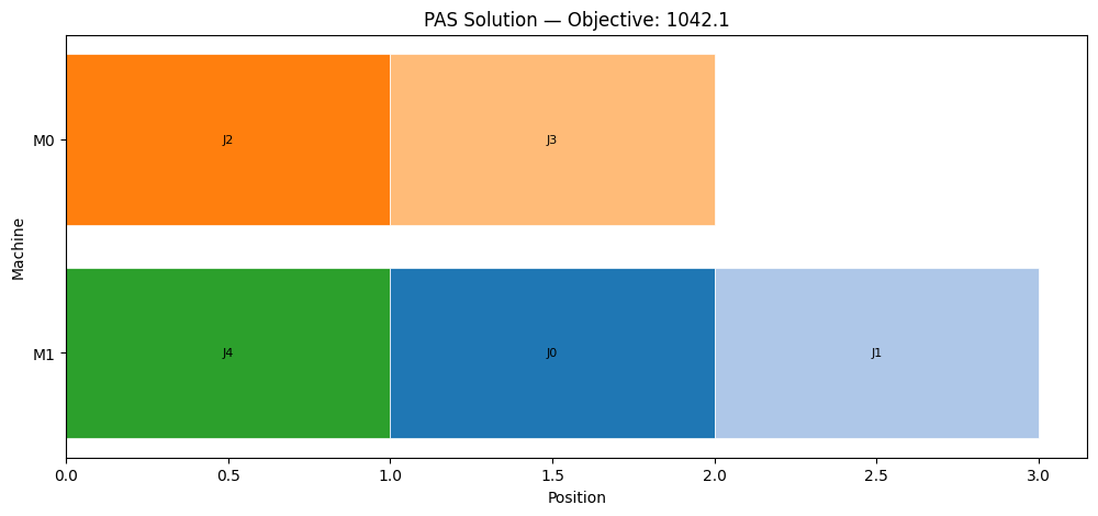
Objective Value: 1042.12
  - Total Job Value: 150.18
  - Total Setup Time: 9.29
  - Load Balance Metric: 2366.03

Machine Loads (Processing Times):
  Machine 0: 34.85
  Machine 1: 33.94

Schedule (Job → Machine @ Position):
  Machine 0: J2 → J3
  Machine 1: J4 → J0 → J1
============================================================

Solution Analysis

The solution output shows: - Schedule by machine: Which jobs are assigned to each machine and in what order - Performance metrics: - Total value achieved (higher is better) - Total setup time (lower is better) - Machine loads (processing time per machine) - Balance metric (sum of squared loads, lower means more balanced) - Weighted objective: The final objective value used for optimization

A good solution balances high value, low setup costs, and even load distribution according to the specified weights.

Working with Collections

Collections provide a powerful abstraction for managing multiple problem instances. This is essential for: - Benchmarking: Comparing solver performance across various problem sizes and characteristics - Parameter studies: Testing how different weight configurations affect solution quality - Batch experiments: Running production-scale optimization campaigns - Statistical analysis: Generating multiple random instances to assess average-case performance

The PasCollection class enables systematic exploration of the problem space.

Generate a Collection

Here we create a collection of instances with varying sizes. The from_random() method generates: - Multiple instances per size configuration (for statistical robustness) - Random but consistent problem data (using seeds for reproducibility) - Instances spanning different scales (5 to 8 jobs in this example) - we use convex model here as the solver is much faster for the selected size

This allows us to study how solution quality and solver performance scale with problem size.

# Generate a collection of random instances
collection = PasCollection.from_random(
    min_size=5,
    max_size=8,
    num_instances=2,  # 2 instances per size
    seed=42,
    formulation_class=PasConvexFormulation,
)

print(f"Collection: {collection.name}")
print(f"Description: {collection.description}")
print(f"Total instances: {len(collection.instances)}\n")

Collection: Random PAS Set 5-8
Description: Random PAS instances with 2 instance(s) per size
Total instances: 8

Batch Formulation

Before solving, we formulate all instances in the collection. This step: - Generates optimization models for each instance - Reports the problem size (number of variables) for each - Allows validation of the formulation before expensive solve operations

The number of variables scales as $\mathcal{O}(J \times M \times J)$ where $J$ is the number of jobs and $M$ is the number of machines (since the maximum number of positions equals $J$).

# Formulate all models in the collection
models = []
for i, instance in enumerate(collection.instances):
    model = instance.formulate()
    models.append(model)
    print(f"Instance {i}: {model.num_variables} variables")

print(f"\nFormulated {len(models)} models!")

Instance 0: 40 variables
Instance 1: 50 variables
Instance 2: 92 variables
Instance 3: 90 variables
Instance 4: 128 variables
Instance 5: 96 variables
Instance 6: 156 variables
Instance 7: 188 variables

Formulated 8 models!

Solving Collections

Now we solve all instances sequentially and collect results. For each instance: 1. Formulate the model 2. Submit to the solver 3. Wait for completion 4. Interpret and store the solution

This demonstrates a basic batch processing workflow. For production use, consider: - Parallel submission: Send multiple jobs simultaneously to leverage backend parallelism - Result caching: Store solutions for later analysis - Error handling: Gracefully handle solver failures or timeouts - Progress tracking: Monitor completion status for long-running batches

solver = SCIP()
solutions = []

for i, instance in enumerate(collection.instances):
    model = instance.formulate()
    print(f"Generated instance {i} with {model.num_variables} variables.")

    job = solver.run(model)
    solutions.append(job.result())  # Wait for job to complete and get solution


print(f"Solved {len(solutions)} instances!")

/Users/maximilianjanetschek/PycharmProjects/luna-usecases/.venv/lib/python3.13/site-packages/rich/live.py:260:
UserWarning: install "ipywidgets" for Jupyter support
  warnings.warn('install "ipywidgets" for Jupyter support')

Generated instance 0 with 40 variables.

2026-05-29 11:36:15 INFO     Sleeping for 5.0 seconds. Waiting and checking a function in a loop.

Generated instance 1 with 50 variables.

2026-05-29 11:36:26 INFO     Sleeping for 5.0 seconds. Waiting and checking a function in a loop.

Generated instance 2 with 92 variables.

2026-05-29 11:36:37 INFO     Sleeping for 5.0 seconds. Waiting and checking a function in a loop.

Generated instance 3 with 90 variables.

2026-05-29 11:36:48 INFO     Sleeping for 5.0 seconds. Waiting and checking a function in a loop.

Generated instance 4 with 128 variables.

2026-05-29 11:36:59 INFO     Sleeping for 5.0 seconds. Waiting and checking a function in a loop.

Generated instance 5 with 96 variables.

2026-05-29 11:37:12 INFO     Sleeping for 5.0 seconds. Waiting and checking a function in a loop.

Generated instance 6 with 156 variables.

2026-05-29 11:37:25 INFO     Sleeping for 5.0 seconds. Waiting and checking a function in a loop.

Generated instance 7 with 188 variables.

2026-05-29 11:37:36 INFO     Sleeping for 5.0 seconds. Waiting and checking a function in a loop.

Solved 8 instances!

Summary and Next Steps

This notebook demonstrated the complete workflow for solving Production Assignment and Scheduling problems:

Problem modeling: Define jobs, machines, and constraints mathematically
Data generation: Create realistic problem instances with configurable parameters
Formulation: Translate the mathematical model into solver-compatible format
Solving: Execute optimization using classical or quantum-classical solvers
Analysis: Interpret results and evaluate solution quality
Scaling: Work with collections for batch processing and benchmarking

Key Takeaways

Multi-objective optimization: PAS balances competing goals (value, setup, balance) via weighted objectives
Constraint programming: Proper constraint modeling ensures feasible, practical schedules
Flexibility: The architecture supports dynamic weight adjustment and multiple solver backends
Scalability: Collections enable systematic study of solver behavior across problem sizes

Extensions to Explore

Weight sensitivity analysis: Study how different $(\alpha, \beta, \gamma)$ values affect solutions
Solver comparison: Benchmark SCIP, SAGA, FlexQAOA, and other solvers
Real-world data: Apply the framework to actual production scheduling scenarios
Advanced constraints: Add time windows, precedence relations, or resource limits
Pre-/Post-processing: for example to decompose into smaller sub problems

Aspect	Position-Based	Routing (Convex)
Variables	\(x_{j,m,n}\) binary (job, machine, position)	\(r_{m,i,j}\) binary (routing edges) + \(c_{m,j}\) continuous (load tracking)
Sequencing	Explicit position slots \(n = 0, 1, 2, \ldots\)	Implicit via predecessor-successor edges
Subtour prevention	"No-gap" constraints	Capacity/MTZ-style constraints
Scalability	Variables grow as \(\mathcal{O}(J \times M \times J)\)	Variables grow as \(\mathcal{O}(M \times J^2)\)