Portfolio Optimization with Investment Bands Example

Download Notebook

Portfolio Optimization with investment bands extends the classical Markowitz mean-variance framework by introducing lower and upper bounds on the allocation of each asset.

The goal is to construct a portfolio that balances expected return and risk while respecting asset-specific investment constraints. The model is formulated as a quadratic optimization problem and discretised using binary variables to make it compatible with QUBO-based solvers.

Objective

The model optimizes the classical mean-variance trade-off:

maximize expected portfolio return
penalize portfolio variance according to a risk aversion parameter λ

Decision Variables

Each asset allocation is represented through binary variables that discretise the continuous investment range within predefined bounds:

binary variables encode discrete allocation levels per asset
continuous investments are reconstructed from these binary encodings

Constraints

Each asset must lie within its investment band \([lower_i, upper_i]\)
The total portfolio investment must not exceed a given budget

Model Assumptions

Expected returns are known and deterministic
Covariance matrix is given and static
No transaction costs or market impact are considered
Asset returns are modeled using a mean-variance approximation
Discretisation is introduced solely for compatibility with QUBO solvers and does not represent a financial assumption

Interpretation

The resulting solution defines a discretised portfolio allocation, which approximates a continuous mean-variance optimal portfolio within the imposed constraints.

import getpass
import os

import numpy as np
from dotenv import load_dotenv
from luna_quantum.algorithms import SCIP

from luna_usecases.portfolio_optimization_with_investment_bands import (
    PoIbtvCollection,
    PoIbtvData,
    PoIbtvFormulation,
    PoIbtvInstance,
)

load_dotenv()
if "LUNA_API_KEY" not in os.environ:
    os.environ["LUNA_API_KEY"] = getpass.getpass("Enter your Luna API key: ")

Create Data

Define 3 assets with log returns, covariance matrix, and investment band constraints.

data = PoIbtvData.from_values(
    log_returns=[0.06, 0.08, 0.03, 0.06, 0.04],
    covariance_matrix=np.array(
        [
            [0.04, 0.01, 0.005, 0.008, 0.006],
            [0.01, 0.09, 0.02, 0.015, 0.01],
            [0.005, 0.02, 0.03, 0.01, 0.007],
            [0.008, 0.015, 0.01, 0.05, 0.012],
            [0.006, 0.01, 0.007, 0.012, 0.04],
        ]
    ),
    investment_bands=[
        (0.0, 0.5),
        (0.0, 0.4),
        (0.0, 0.6),
        (0.0, 0.3),
        (0.0, 0.1),
    ],
    risk_aversion=1.2,
    max_budget=1.0,
    n_bits=3,
)

print(data.to_string())

Portfolio Optimization with Investment Bands Data:
  Number of assets: 5
  Discretization bits: 3
  Risk aversion:     1.2
  Max budget:        1.0

Assets:
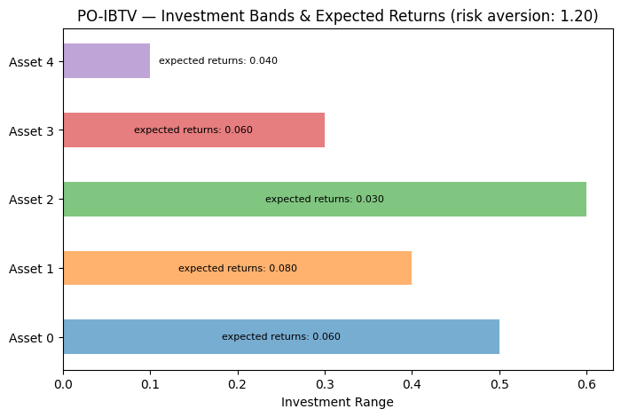
  Asset 0: return=0.0600, band=[0.0000, 0.5000]
  Asset 1: return=0.0800, band=[0.0000, 0.4000]
  Asset 2: return=0.0300, band=[0.0000, 0.6000]
  Asset 3: return=0.0600, band=[0.0000, 0.3000]
  Asset 4: return=0.0400, band=[0.0000, 0.1000]

Plot Data

Visualize asset returns and investment band constraints.

data.plot()

<Axes: title={'center': 'PO-IBTV — Investment Bands & Expected Returns (risk aversion: 1.20)'}, xlabel='Investment Range'>

Create Formulation

Allocate assets within investment bands while constraining portfolio volatility.

formulation = PoIbtvFormulation()
print(formulation.to_string(data))

PO Investment Bands Formulation:
  Assets: 5
  Bits per asset: 3
  Risk aversion: 1.2000
  Max budget: 1.0

Decision Variables:
  x[i,q] in {0,1} for i = 0, ..., 4, q = 0, ..., 2
  x[i,q] encodes the binary decomposition of asset i allocation
  Total: 15 binary variables

Objective:
  maximize sum_i return[i] * investment[i]
           - risk_aversion * sum_(Undefined, Undefined) sigma[i,j] * investment[i] * investment[j]

Constraints:
  1. Budget constraint (1 constraint):
     sum_i investment[i] <= 1.0

Create Instance

Combine data and formulation into a solvable instance.

instance = PoIbtvInstance(data=data, formulation=formulation)
print(instance.to_string())

Data:Portfolio Optimization with Investment Bands Data:
  Number of assets: 5
  Discretization bits: 3
  Risk aversion:     1.2
  Max budget:        1.0

Assets:
  Asset 0: return=0.0600, band=[0.0000, 0.5000]
  Asset 1: return=0.0800, band=[0.0000, 0.4000]
  Asset 2: return=0.0300, band=[0.0000, 0.6000]
  Asset 3: return=0.0600, band=[0.0000, 0.3000]
  Asset 4: return=0.0400, band=[0.0000, 0.1000]
Formulation:PO Investment Bands Formulation:
  Assets: 5
  Bits per asset: 3
  Risk aversion: 1.2000
  Max budget: 1.0

Decision Variables:
  x[i,q] in {0,1} for i = 0, ..., 4, q = 0, ..., 2
  x[i,q] encodes the binary decomposition of asset i allocation
  Total: 15 binary variables

Objective:
  maximize sum_i return[i] * investment[i]
           - risk_aversion * sum_(Undefined, Undefined) sigma[i,j] * investment[i] * investment[j]

Constraints:
  1. Budget constraint (1 constraint):
     sum_i investment[i] <= 1.0

Formulate Model

Translate the instance into a mathematical optimization model.

model = instance.formulate()

Solve and Interpret

Solve the model with SCIP and interpret the raw result into a use-case-specific solution.

scip = SCIP()
job = scip.run(model)
sol = job.result()
uc_solution = instance.interpret(sol)
print(uc_solution.to_string())

/Users/maximilianjanetschek/PycharmProjects/luna-usecases/.venv/lib/python3.13/site-packages/rich/live.py:260:
UserWarning: install "ipywidgets" for Jupyter support
  warnings.warn('install "ipywidgets" for Jupyter support')

Portfolio Optimization with Investment Bands Solution:
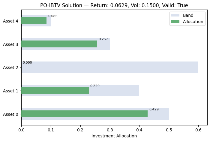
  Status: VALID
  Asset 0: 0.428571
  Asset 1: 0.228571
  Asset 2: 0.000000
  Asset 3: 0.257143
  Asset 4: 0.085714
  Portfolio Return:     0.062857
  Portfolio Volatility: 0.149988

Plot Solution

Visualize the optimal solution.

uc_solution.plot(data)

<Axes: title={'center': 'PO-IBTV Solution — Return: 0.0629, Vol: 0.1500, Valid: True'}, xlabel='Investment Allocation'>

Collections

Generate a benchmark collection of random instances for batch processing.

collection = PoIbtvCollection.from_random(min_assets=2, max_assets=5, n_bits=3, num_instances=1, seed=42)
model = collection.instances[0].formulate()
print(model)

Model: portfolio_optimization_with_investment_bands<portfolio_optimization_with_investment_bands>
Maximize
  -0.0000009342133667775807 * x_0_0 * x_0_1
  - 0.0000018684267335551613 * x_0_0 * x_0_2
  - 0.0000020134260094036983 * x_0_0 * x_1_0
  - 0.000004026852018807397 * x_0_0 * x_1_1
  - 0.000008053704037614793 * x_0_0 * x_1_2
  - 0.0000037368534671103227 * x_0_1 * x_0_2
  - 0.000004026852018807397 * x_0_1 * x_1_0
  - 0.000008053704037614793 * x_0_1 * x_1_1
  - 0.000016107408075229586 * x_0_1 * x_1_2
  - 0.000008053704037614793 * x_0_2 * x_1_0
  - 0.000016107408075229586 * x_0_2 * x_1_1
  - 0.00003221481615045917 * x_0_2 * x_1_2
  - 0.0000625820943834702 * x_1_0 * x_1_1
  - 0.0001251641887669404 * x_1_0 * x_1_2
  - 0.0002503283775338808 * x_1_1 * x_1_2 + 0.003015164703338624 * x_0_0
  + 0.00602986229999386 * x_0_1 + 0.012057856173254165 * x_0_2
  + 0.0010399817128410014 * x_1_0 + 0.002048672378490268 * x_1_1
  + 0.003972180568213595 * x_1_2
Subject To
  budget: 0.0681327191380834 * x_0_0 + 0.1362654382761668 * x_0_1
    + 0.2725308765523336 * x_0_2 + 0.06097222791097653 * x_1_0
    + 0.12194445582195305 * x_1_1 + 0.2438889116439061 * x_1_2 <=
    0.9385909856669729
Binary
  x_0_0 x_0_1 x_0_2 x_1_0 x_1_1 x_1_2