Benchmark Multiple Use Cases with LunaBench
In this tutorial, you'll learn how to combine several problem collections from the use case library into a single LunaBench benchmark, run a set of solvers against all of them at once, and then break the results down per use case and per problem size. We will use the closely related Maximum Independent Set (MIS) and Minimum Vertex Cover (MVC) problems as our two use cases and compare Simulated Annealing, Tabu Search and QAOA on them.
What You'll Learn
By the end of this tutorial, you will:
- Generate reproducible problem collections for multiple use cases with luna_usecases
- Collect the models of all collections in one LunaBench ModelSet and label each model with its use case as a feature label
- Assemble a Benchmark from algorithms, features, metrics and plots and run it
- Group the built-in plots by use case, and analyze the results further as a DataFrame
Setup
Before starting, make sure that the following dependencies are installed:
%%capture
# Install the python packages that are needed for the notebook
%pip install --upgrade pip
%pip install luna_quantum luna_usecases "luna-bench[pre-defined]" pandas seaborn --upgrade
Next, authenticate with your personal API key (LUNA_API_KEY) to securely access LunaSolve's services. If this feels unfamiliar to you, you can make a quick revision in the Get Started Guide. The two LB_LOG_* variables keep LunaBench's own logging as quiet as the LunaSolve one.
import os
import getpass

os.environ["LUNA_LOG_DEFAULT_LEVEL"] = "WARNING"
os.environ["LUNA_LOG_DISABLE_SPINNER"] = "true"
os.environ["LB_LOG_DEFAULT_LEVEL"] = "WARNING"
os.environ["LB_LOG_DISABLE_SPINNER"] = "true"

if "LUNA_API_KEY" not in os.environ:
    # Prompt securely for the key if not already set
    os.environ["LUNA_API_KEY"] = getpass.getpass("Enter your Luna API key: ")
from luna_quantum import LunaSolve

LunaSolve.authenticate(os.environ["LUNA_API_KEY"])
ls = LunaSolve()
Step 1: Generate the Use Case Collections
Every use case in the library ships a Collection class with generator methods that create a whole family of random problem instances at once. This is exactly what a benchmark needs: many models of the same kind at increasing sizes, rather than a single hand-built graph.
We generate two collections here:
- Maximum Independent Set (MIS): pick the largest set of nodes such that no two of them share an edge. A maximization problem with one constraint per edge.
- Minimum Vertex Cover (MVC): pick the smallest set of nodes such that every edge touches at least one of them. A minimization problem, and in fact the complement of MIS on the same graph.
Both generators take a node range and the number of instances per size. With min_nodes=5, max_nodes=8 and num_instances=2 each collection therefore contains \(4 \times 2 = 8\) graphs, 16 models in total. Setting seed makes the generated graphs reproducible.
We keep the graphs small and sparse on purpose. QAOA runs on an unconstrained (QUBO) version of each model, and the conversion adds one slack qubit per edge constraint, so a graph needs roughly nodes + edges qubits. IBM's Aer simulator supports at most 18 of them, which an 8-node graph with edge_prob=0.3 stays safely below.
from luna_usecases.max_independent_set import MaxIndependentSetCollection
from luna_usecases.minimum_vertex_cover import MinimumVertexCoverCollection

SEED = 42

collections = {
    "MIS": MaxIndependentSetCollection.from_random(
        min_nodes=5, max_nodes=8, num_instances=2, edge_prob=0.3, seed=SEED
    ),
    "MVC": MinimumVertexCoverCollection.from_random(
        min_nodes=5, max_nodes=8, num_instances=2, edge_prob=0.3, seed=SEED
    ),
}

for label, collection in collections.items():
    print(f"{label}: {len(collection.instances)} instances")
MIS: 8 instances
MVC: 8 instances
Step 2: Collect All Models in One ModelSet
A LunaBench ModelSet is a named, persisted collection of models. Every algorithm in a benchmark runs against every model of its model set, so putting the models of both collections into the same set is all we need to benchmark across use cases. collection.get_models() formulates every instance into an optimization Model for us.
Once the models sit in one set, however, LunaBench no longer knows which collection each of them came from. To get that information back into the results, we define a lookup feature. Regular features compute a property from the model itself, like its number of variables. A lookup feature instead serves a value that we assign to each model by hand, which is the right tool for labels such as a use case, a data source or a difficulty rating. Subclassing BaseValueLookupFeature[str] and registering the class with the @feature decorator is all it takes; the feature is then filled with add_model() while we build the model set.
from luna_bench import ModelSet
from luna_bench.custom import BaseValueLookupFeature, feature


@feature
class UseCaseFeature(BaseValueLookupFeature[str]):
    """The use case a model was generated from."""


model_set = ModelSet.create("mis-vs-mvc")
use_case = UseCaseFeature()

for label, collection in collections.items():
    models = collection.get_models()
    model_set.add(models)
    for model in models:
        use_case.add_model(model, label)

print(f"{len(model_set.models)} models in the set, for example:")
for metadata in model_set.models[:3]:
    print(f"  {metadata.name}")
16 models in the set, for example:
  max_independent_set<s42_n5_i0>
  max_independent_set<s42_n5_i1>
  max_independent_set<s42_n6_i0>
Persistence. Model sets and benchmarks are stored in a local SQLite database (
./benchmark_databy default). Re-running this cell loads the existing set instead of creating a duplicate, and adding the same models again is a no-op because models are deduplicated by their hash.
Step 3: Assemble the Benchmark
A Benchmark ties together four kinds of components, which LunaBench runs in this order:
- Features extract properties of each model before solving, e.g. the number of variables or the optimal objective value.
- Algorithms are the solvers being compared. Any LunaSolve algorithm can be added directly.
- Metrics score each
(algorithm, model)result, optionally using the features. - Plots visualize the collected metrics.
We compare three algorithms: Simulated Annealing and Tabu Search, two classical heuristics, and QAOA on IBM's Aer simulator with two layers. Each algorithm is registered under a short name that will show up in every result table and plot.
from luna_bench import Benchmark
from luna_quantum.algorithms import QAOA, SimulatedAnnealing, TabuSearch
from luna_quantum.backends import AerSimulator

bench = Benchmark.open("mis-vs-mvc")
bench.set_modelset(model_set)

bench.add_algorithm("simulated-annealing", SimulatedAnnealing(num_reads=100))
bench.add_algorithm("tabu-search", TabuSearch(num_reads=100))
bench.add_algorithm(
    "qaoa",
    QAOA(
        backend=AerSimulator(backend_type="simulator", aer_config=None),
        reps=2,
        shots=1024,
    ),
)

print("Algorithms:", [entry.name for entry in bench.algorithms])
Algorithms: ['simulated-annealing', 'tabu-search', 'qaoa']
Next come the features and metrics. Besides our use_case lookup feature we need two more. The approximation ratio measures how close the expected objective value of an algorithm's samples is to the optimum, so it needs to know that optimum: the OptSolFeature computes it for every model with a local SCIP solve. The VarNumberFeature records the problem size, which we want to look at later. The feasibility ratio tells us which fraction of the samples satisfied all constraints, which is particularly interesting for MIS and MVC since their constraints are handled through penalty terms once the model is converted to QUBO form.
Fill lookup features before adding them. The benchmark stores a feature's configuration the moment it is added. Models registered on
use_caseafterbench.add_feature()would never reach the run.
from luna_bench.features import OptSolFeature, VarNumberFeature
from luna_bench.metrics import ApproximationRatio, FeasibilityRatio, Runtime

bench.add_feature("use-case", use_case)
bench.add_feature("optimal", OptSolFeature())
bench.add_feature("num-vars", VarNumberFeature())

bench.add_metric("approx-ratio", ApproximationRatio())
bench.add_metric("feasibility", FeasibilityRatio())
bench.add_metric("runtime", Runtime())

print("Features:", [entry.name for entry in bench.features])
print("Metrics:", [entry.name for entry in bench.metrics])
Features: ['use-case', 'optimal', 'num-vars']
Metrics: ['approx-ratio', 'feasibility', 'runtime']
Every metric has a matching built-in bar plot, and by default each of them draws one bar per algorithm, averaged over all models. That would hide the difference between the two use cases, which is what we set out to investigate. Each bar plot therefore takes two dimensions: x decides what the bars are, and grouping splits each bar into a group of bars. Both accept the same kinds of dimension, so it is only a question of which role we assign:
AlgorithmDimension()andModelDimension()organize by the columns every result carries.FeatureDimension(SomeFeature)organizes by the value a feature assigned to each model, which is where ourUseCaseFeaturecomes in.ParameterDimension("reps")organizes by the setting an algorithm was run with.
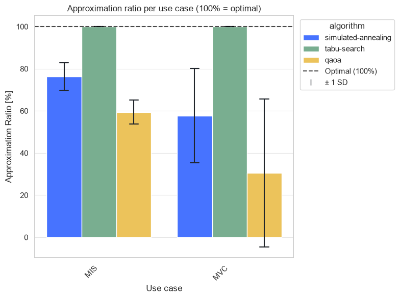
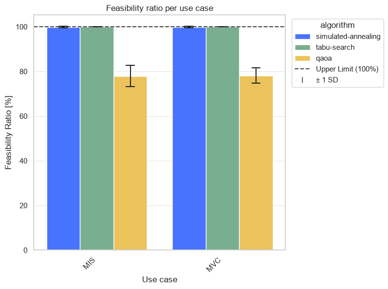
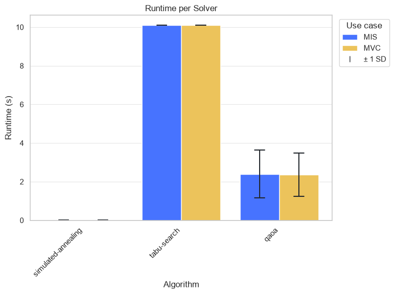
For the approximation and feasibility ratios we put the use cases on the x-axis and colour the bars by algorithm. For the runtime we keep the algorithms on the x-axis and split each bar by use case, to show the other role of the same dimension.
from luna_bench.plots import (
    AlgorithmDimension,
    ApproximationRatioPlot,
    FeasibilityRatioPlot,
    FeatureDimension,
    Figure,
    RuntimePlot,
)

by_use_case = FeatureDimension(UseCaseFeature, label="Use case")

bench.add_plot(
    "approx-ratio-per-use-case",
    ApproximationRatioPlot(
        x=by_use_case,
        grouping=AlgorithmDimension(),
        figure=Figure(
            filename="approximation_ratio",
            title="Approximation ratio per use case (100% = optimal)",
        ),
    ),
)
bench.add_plot(
    "feasibility-per-use-case",
    FeasibilityRatioPlot(
        x=by_use_case,
        grouping=AlgorithmDimension(),
        figure=Figure(filename="feasibility_ratio", title="Feasibility ratio per use case"),
    ),
)
bench.add_plot(
    "runtime-per-algorithm",
    RuntimePlot(grouping=by_use_case),
)

print("Plots:", [entry.name for entry in bench.plots])
Plots: ['approx-ratio-per-use-case', 'feasibility-per-use-case', 'runtime-per-algorithm']
Step 4: Run the Benchmark
bench.run() executes the full pipeline: features, then all 3 algorithms on all 16 models, then the metrics and finally the plots. The algorithm stage submits the solve jobs to LunaSolve and waits for their results, so this cell will take a few minutes, with the QAOA simulations making up most of it. The plots are shown once the run is complete and are also saved as PNG files next to the benchmark's database.
A few things are worth reading off these charts:
- The approximation ratio is computed from the expectation value of all samples an algorithm returned, not from its best one. Tabu Search concentrates its samples on the optimum and scores 100% on both use cases, while Simulated Annealing and QAOA spread theirs out and score lower, even though their best samples are often optimal too. The wide error bars on MVC show that this spread differs a lot from graph to graph.
- MIS and MVC share the same kind of edge constraints, but they pull in opposite directions: for MIS the objective rewards adding nodes, so violating a constraint is tempting, whereas for MVC the objective rewards removing nodes and the constraints have to keep enough of them in. The two heuristics return feasible samples almost exclusively for both, whereas about a fifth of QAOA's samples violate a constraint, which drags its approximation ratio down further.
- Grouping the runtime by use case checks that neither problem is systematically more expensive to solve. Note that Tabu Search takes the same time on every model, which tells us it ran to its time budget rather than to convergence.
Step 5: Analyze the Results as a DataFrame
The built-in plots cover the per-use-case comparison, but any further slicing is easiest on the raw results. bench.to_dataframe() returns one row per (algorithm, model) pair. Every metric and feature contributes its result fields as "<name>/<field>" columns, where <name> is the name we registered the component under, so the use case of each row is readily available in the use-case/value column.
df = bench.to_dataframe()

columns = [
    "algorithm",
    "model",
    "use-case/value",
    "num-vars/var_number",
    "approx-ratio/approximation_ratio",
    "feasibility/feasibility_ratio",
    "runtime/runtime_seconds",
]
df[columns].head()
| algorithm | model | use-case/value | num-vars/var_number | approx-ratio/approximation_ratio | feasibility/feasibility_ratio | runtime/runtime_seconds | |
|---|---|---|---|---|---|---|---|
| 0 | simulated-annealing | max_independent_set<s42_n5_i0> | MIS | 5 | 0.800000 | 1.00 | 0.016543 |
| 1 | simulated-annealing | max_independent_set<s42_n5_i1> | MIS | 5 | 0.856667 | 1.00 | 0.013254 |
| 2 | simulated-annealing | max_independent_set<s42_n6_i0> | MIS | 6 | 0.662500 | 1.00 | 0.021991 |
| 3 | simulated-annealing | max_independent_set<s42_n6_i1> | MIS | 6 | 0.833333 | 0.99 | 0.022143 |
| 4 | simulated-annealing | max_independent_set<s42_n7_i0> | MIS | 7 | 0.752500 | 1.00 | 0.025309 |
A groupby over use case and algorithm condenses the 48 rows into the same numbers the plots are drawn from, in one table.
summary = (
    df.groupby(["use-case/value", "algorithm"])[
        [
            "approx-ratio/approximation_ratio",
            "feasibility/feasibility_ratio",
            "runtime/runtime_seconds",
        ]
    ]
    .mean()
    .round(3)
)
summary
| approx-ratio/approximation_ratio | feasibility/feasibility_ratio | runtime/runtime_seconds | ||
|---|---|---|---|---|
| use-case/value | algorithm | |||
| MIS | qaoa | 0.594 | 0.780 | 2.396 |
| simulated-annealing | 0.763 | 0.999 | 0.022 | |
| tabu-search | 1.000 | 1.000 | 10.102 | |
| MVC | qaoa | 0.305 | 0.781 | 2.362 |
| simulated-annealing | 0.577 | 0.999 | 0.022 | |
| tabu-search | 1.000 | 1.000 | 10.103 |
Step 6: Plot the Approximation Ratio Against Problem Size
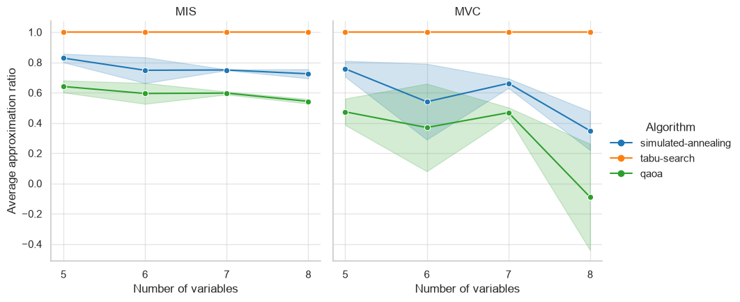
As a last insight, we group by problem size as well. The num-vars/var_number feature gives the number of variables of every model, which for MIS and MVC equals the number of nodes. A seaborn line plot on the DataFrame with one panel per use case and one line per algorithm shows how the approximation ratio develops as the graphs grow, and whether the heuristics and QAOA degrade at the same pace.
import matplotlib.pyplot as plt
import seaborn as sns

ALGORITHM_ORDER = ["simulated-annealing", "tabu-search", "qaoa"]
ALGORITHM_COLORS = {
    "simulated-annealing": "#1f77b4",
    "tabu-search": "#ff7f0e",
    "qaoa": "#2ca02c",
}

grid = sns.relplot(
    df,
    kind="line",
    x="num-vars/var_number",
    y="approx-ratio/approximation_ratio",
    hue="algorithm",
    hue_order=ALGORITHM_ORDER,
    palette=ALGORITHM_COLORS,
    col="use-case/value",
    col_order=list(collections),
    marker="o",
    height=4.5,
    aspect=1,
)
grid.set_axis_labels("Number of variables", "Average approximation ratio")
grid.set_titles("{col_name}")
grid.set(xticks=sorted(df["num-vars/var_number"].unique()))
grid.legend.set_title("Algorithm")
plt.show()
Well done! You have benchmarked three algorithms across two use cases with a single Benchmark, labelled every model with a lookup feature, and used that label both to group the built-in plots and to slice the results DataFrame. Since the whole benchmark is persisted, you can come back to it at any time with Benchmark.load("mis-vs-mvc"), add another algorithm, metric or plot, and re-run only the stages you need.
Next Steps
- Add a third collection, for example
MaxCliqueCollectionfromluna_usecases.max_clique, to the same model set. Only thecollectionsdictionary needs an extra entry. - Register QAOA twice with different depths, e.g.
reps=2andreps=4, and compare them withApproximationRatioPlot(grouping=ParameterDimension("reps")). - Turn the size-scaling chart into a reusable component with a custom plot, or score the results with your own custom metric.
- Explore the other problems in the use case library.